1 Week 1: A Primer on Using Text as Data
1.1 Setup
For this first example, we will replicate (and extend) Mendenhall’s (1887) and Mendenhall’s (1901) studies of word-length distribution.
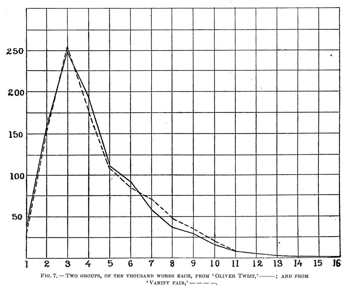
Figure 1.1: From Mendenhall (1987) - The Characteristic Curves of Composition.
First we load the packages that we’ll be using:
library(tidyverse) # for wrangling data
library(tidylog) # to know what we are wrangling
library(tidytext) # for 'tidy' manipulation of text data
library(wesanderson) # to prettify
library(gutenbergr) # to get some books
library(kableExtra) # for displaying data in html format (relevant for formatting this worksheet mainly)
1.2 Get Data
Mendenhall (1887) argued that “every writer makes use of a vocabulary which is peculiar to himself, and the character of which does not materially change from year to year during his productive,” and that one of these characteristics was the length of words. Mendenhall (1901) takes this further, and suggests that, given this assumption, Shakespeare and Bacon were not the same person2.
Let’s get a corpus–a collection of documents–that we can analyze. We can search the Gutenberg repository and create a corpus with some selected work.
gutenberg_metadata %>%
  filter(author == "Wilde, Oscar")
## # A tibble: 66 × 8
## gutenberg_id title author gutenberg_author_id language gutenberg_bookshelf
## <int> <chr> <chr> <int> <chr> <chr>
## 1 174 The Pic… Wilde… 111 en "Gothic Fiction/Mo…
## 2 301 The Bal… Wilde… 111 en ""
## 3 773 Lord Ar… Wilde… 111 en "Contemporary Revi…
## 4 774 Essays … Wilde… 111 en ""
## 5 790 Lady Wi… Wilde… 111 en ""
## 6 844 The Imp… Wilde… 111 en "Plays"
## 7 854 A Woman… Wilde… 111 en "Plays"
## 8 873 A House… Wilde… 111 en "Opera"
## 9 875 The Duc… Wilde… 111 en ""
## 10 885 An Idea… Wilde… 111 en "Plays"
## # ℹ 56 more rows
## # ℹ 2 more variables: rights <chr>, has_text <lgl>1.3 Word Length in Wilde’s Corpus
That’s a lot of Wilde! Let’s focus on four plays: “The Importance of Being Earnest”, “A Woman of No Importance”, “Lady Windermere’s Fan”, and “An Ideal Husband”. We can download all of these plays using their ID number:
wilde <- gutenberg_download(c(790,844, 854, 885),
                            meta_fields = c("title","author"))
print(n=25,wilde[c(51:75),])
## # A tibble: 25 × 4
## gutenberg_id text title author
## <int> <chr> <chr> <chr>
## 1 790 "" Lady Winderm… Wilde…
## 2 790 "" Lady Winderm… Wilde…
## 3 790 "THE PERSONS OF THE PLAY" Lady Winderm… Wilde…
## 4 790 "" Lady Winderm… Wilde…
## 5 790 "" Lady Winderm… Wilde…
## 6 790 "Lord Windermere" Lady Winderm… Wilde…
## 7 790 "" Lady Winderm… Wilde…
## 8 790 "Lord Darlington" Lady Winderm… Wilde…
## 9 790 "" Lady Winderm… Wilde…
## 10 790 "Lord Augustus Lorton" Lady Winderm… Wilde…
## 11 790 "" Lady Winderm… Wilde…
## 12 790 "Mr. Dumby" Lady Winderm… Wilde…
## 13 790 "" Lady Winderm… Wilde…
## 14 790 "Mr. Cecil Graham" Lady Winderm… Wilde…
## 15 790 "" Lady Winderm… Wilde…
## 16 790 "Mr. Hopper" Lady Winderm… Wilde…
## 17 790 "" Lady Winderm… Wilde…
## 18 790 "Parker, Butler" Lady Winderm… Wilde…
## 19 790 "" Lady Winderm… Wilde…
## 20 790 " * * * * *" Lady Winderm… Wilde…
## 21 790 "" Lady Winderm… Wilde…
## 22 790 "Lady Windermere" Lady Winderm… Wilde…
## 23 790 "" Lady Winderm… Wilde…
## 24 790 "The Duchess of Berwick" Lady Winderm… Wilde…
## 25 790 "" Lady Winderm… Wilde…The unit of analysis is something like a line. We are interested in each word—also known as token—and their lengths in each play. We will clean some of the unwanted text—text that will only add noise to our analysis—and then count the number of words.
wilde <- wilde %>%
  # Some housekeeping
  mutate(title = ifelse(str_detect(title,"Importance of Being"),"The Importance of Being Earnest", title)) %>%
  # Filter out all empty rows
  filter(text != "") %>%
  # This is a play. The name of each character before they speak
  filter(str_detect(text,"[A-Z]{3,}")==FALSE)
## mutate: changed 3,884 values (27%) of 'title' (0 new NA)## filter: removed 4,232 rows (29%), 10,303 rows remaining## filter: removed 4,208 rows (41%), 6,095 rows remaining## # A tibble: 25 × 4
## gutenberg_id text title author
## <int> <chr> <chr> <chr>
## 1 790 "tea-table L._ _Window opening on to terrace L._ … Lady… Wilde…
## 2 790 "home to any one who calls." Lady… Wilde…
## 3 790 " … Lady… Wilde…
## 4 790 "he’s come." Lady… Wilde…
## 5 790 "hands with you. My hands are all wet with these … Lady… Wilde…
## 6 790 "lovely? They came up from Selby this morning." Lady… Wilde…
## 7 790 "table_.] And what a wonderful fan! May I look a… Lady… Wilde…
## 8 790 "everything. I have only just seen it myself. It… Lady… Wilde…
## 9 790 "present to me. You know to-day is my birthday?" Lady… Wilde…
## 10 790 "life, isn’t it? That is why I am giving this par… Lady… Wilde…
## 11 790 "down. [_Still arranging flowers_.]" Lady… Wilde…
## 12 790 "birthday, Lady Windermere. I would have covered … Lady… Wilde…
## 13 790 "front of your house with flowers for you to walk … Lady… Wilde…
## 14 790 "you." Lady… Wilde…
## 15 790 " … Lady… Wilde…
## 16 790 "Foreign Office. I am afraid you are going to ann… Lady… Wilde…
## 17 790 "with her pocket-handkerchief_, _goes to tea-table… Lady… Wilde…
## 18 790 "Won’t you come over, Lord Darlington?" Lady… Wilde…
## 19 790 "miserable, Lady Windermere. You must tell me wha… Lady… Wilde…
## 20 790 "table L._]" Lady… Wilde…
## 21 790 "whole evening." Lady… Wilde…
## 22 790 "that the only pleasant things to pay _are_ compli… Lady… Wilde…
## 23 790 "things we _can_ pay." Lady… Wilde…
## 24 790 "You mustn’t laugh, I am quite serious. I don’t l… Lady… Wilde…
## 25 790 "don’t see why a man should think he is pleasing a… Lady… Wilde…Now, we can change our unit of analysis to the token:
wilde_words <- wilde %>%
  # take the column text and divide it by words
  unnest_tokens(word, text) %>%
  # Remove some characters that add noise
  mutate(word = str_remove_all(word, "\\_"))
## mutate: changed 1,225 values (2%) of 'word' (0 new NA)
wilde_words## # A tibble: 60,465 × 4
## gutenberg_id title author word
## <int> <chr> <chr> <chr>
## 1 790 Lady Windermere's Fan Wilde, Oscar by
## 2 790 Lady Windermere's Fan Wilde, Oscar sixteenth
## 3 790 Lady Windermere's Fan Wilde, Oscar edition
## 4 790 Lady Windermere's Fan Wilde, Oscar first
## 5 790 Lady Windermere's Fan Wilde, Oscar published
## 6 790 Lady Windermere's Fan Wilde, Oscar 1893
## 7 790 Lady Windermere's Fan Wilde, Oscar first
## 8 790 Lady Windermere's Fan Wilde, Oscar issued
## 9 790 Lady Windermere's Fan Wilde, Oscar by
## 10 790 Lady Windermere's Fan Wilde, Oscar methuen
## # ℹ 60,455 more rowsThat’s a lot of words! We will now create a column for word length, and then count the number of words by length (by play!).
wilde_words_ct <- wilde_words %>%
  # Length of each word
  mutate(word_length = str_length(word)) %>%
  # Group by word_length and count how many
  group_by(word_length,title) %>%
  mutate(total_word_length = n()) %>%
  # Keep relevant
  distinct(word_length,title,.keep_all=T) %>%
  select(word_length,title,author,total_word_length)
## mutate: new variable 'word_length' (integer) with 17 unique values and 0% NA## group_by: 2 grouping variables (word_length, title)## mutate (grouped): new variable 'total_word_length' (integer) with 58 unique values and 0% NA## distinct (grouped): removed 60,403 rows (>99%), 62 rows remaining## select: dropped 2 variables (gutenberg_id, word)Let’s see the distribution by play:
wilde_words_ct %>%
  ggplot(aes(y=total_word_length,x=word_length,color=title)) +
  geom_point(alpha=0.8) +
  geom_line(alpha=0.8) +
  scale_color_manual(values = wes_palette("Royal2")) +
  theme_minimal() +
  theme(legend.position = "right") +
  labs(x="Length", y = "Total Number of Words", color = "")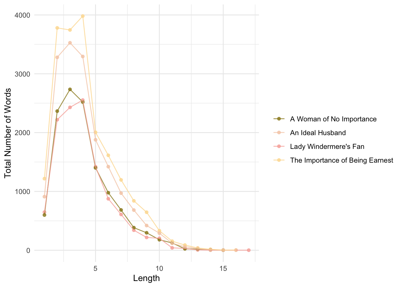
This is a problem. Why?
Here is a solution (proposed by Mendenhall):
wilde_words %>%
  group_by(title) %>%
  slice_sample(n=10000) %>%
  mutate(word_length = str_length(word),
         median_word_length = median(word_length)) %>%
  group_by(word_length,title) %>%
  mutate(total_word_length = n()) %>%
  distinct(word_length,title,.keep_all=T) %>%
  select(word_length,title,author,total_word_length,median_word_length) %>%
  ggplot(aes(y=total_word_length,x=word_length,color=title)) +
  geom_point(alpha=0.8) +
  geom_line(alpha=0.8) +
  geom_vline(aes(xintercept = median_word_length,color=title,linetype = title))+
  scale_color_manual(values = wes_palette("Royal2")) +
  theme_minimal() +
  theme(legend.position = "right") +
  labs(x="Length", y = "Total Number of Words", color = "", linetype = "",
       caption = "Note: Line type shows median word length.")
## group_by: one grouping variable (title)## slice_sample (grouped): removed 20,465 rows (34%), 40,000 rows remaining## mutate (grouped): new variable 'word_length' (integer) with 17 unique values and 0% NA## new variable 'median_word_length' (double) with one unique value and 0% NA## group_by: 2 grouping variables (word_length, title)## mutate (grouped): new variable 'total_word_length' (integer) with 56 unique values and 0% NA## distinct (grouped): removed 39,940 rows (>99%), 60 rows remaining## select: dropped 2 variables (gutenberg_id, word)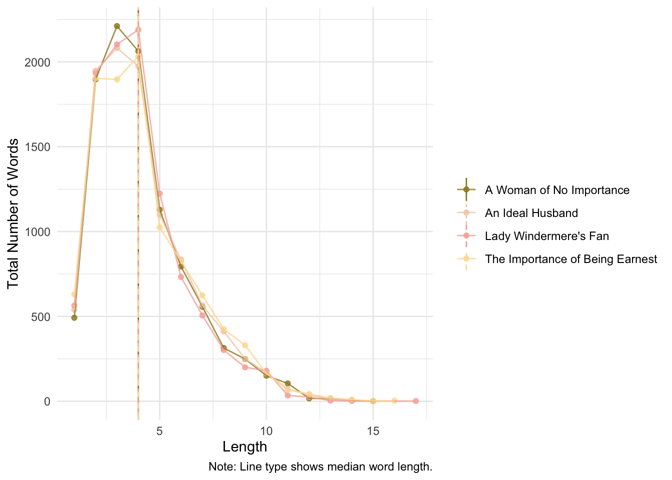
Would you look at that. Mendenhall was into something: an author has a mark in terms of word length distribution. For Wilde, there is no observable change across time (each play was published in different years). But, what happens when we compare Wilde’s mark with Shakespeare’s? Let’s choose four plays (at random) by Shakespeare: A Midsummer Night’s Dream, The Merchant of Venice, Much Ado about Nothing, and The Tempest.
1.4 Comparing Shakespeare and Wilde
shakes <- gutenberg_download(c(1520,2242,2243,2235),
                             meta_fields = c("title","author"))
print(n=25,shakes[c(51:75),])
## # A tibble: 25 × 4
## gutenberg_id text title author
## <int> <chr> <chr> <chr>
## 1 1520 "Leon." Much… Shake…
## 2 1520 "How many gentlemen have you lost in this action?" Much… Shake…
## 3 1520 "" Much… Shake…
## 4 1520 "Mess." Much… Shake…
## 5 1520 "But few of any sort, and none of name." Much… Shake…
## 6 1520 "" Much… Shake…
## 7 1520 "Leon." Much… Shake…
## 8 1520 "A victory is twice itself when the achiever bring… Much… Shake…
## 9 1520 "numbers. I find here that Don Pedro hath bestowe… Much… Shake…
## 10 1520 "a young Florentine, called Claudio." Much… Shake…
## 11 1520 "" Much… Shake…
## 12 1520 "Mess." Much… Shake…
## 13 1520 "Much deserved on his part, and equally remembered… Much… Shake…
## 14 1520 "He hath borne himself beyond the promise of his a… Much… Shake…
## 15 1520 "in the figure of a lamb, the feats of a lion: he … Much… Shake…
## 16 1520 "better bettered expectation than you must expect … Much… Shake…
## 17 1520 "you how." Much… Shake…
## 18 1520 "" Much… Shake…
## 19 1520 "Leon." Much… Shake…
## 20 1520 "He hath an uncle here in Messina will be very muc… Much… Shake…
## 21 1520 "" Much… Shake…
## 22 1520 "Mess." Much… Shake…
## 23 1520 "I have already delivered him letters, and there a… Much… Shake…
## 24 1520 "joy in him; even so much that joy could not show … Much… Shake…
## 25 1520 "enough without a badge of bitterness." Much… Shake…This text is cleaner than Wilde’s corpus, so we will leave it as is. Also, it is harder to systematically remove the name of the person speaking. Is this a problem? Why? Why not?
We can put together both corpora and see differences in the distributions of word length.
shakes_words <- shakes %>%
  # Filter out all empty rows
  filter(text != "") %>%
  # This is a play. The name of each character before they speak
  filter(str_detect(text,"[A-Z]{3,}")==FALSE) %>%
  # take the column text and divide it by words
  unnest_tokens(word, text)
## filter: removed 3,088 rows (22%), 11,135 rows remaining## filter: removed 31 rows (<1%), 11,104 rows remaining
# Bind both word dfs
words <- rbind.data.frame(shakes_words,wilde_words)

# Count words etc.
words %>%
  group_by(title,author) %>%
  slice_sample(n=10000) %>%
  mutate(word_length = str_length(word),
         median_word_length = median(word_length)) %>%
  group_by(word_length,title,author) %>%
  mutate(total_word_length = n()) %>%
  distinct(word_length,title,.keep_all=T) %>%
  select(word_length,title,author,total_word_length,median_word_length) %>%
  ggplot(aes(y=total_word_length,x=word_length,color=author,group=title)) +
  geom_point(alpha=0.8) +
  geom_line(alpha=0.8) +
  scale_color_manual(values = wes_palette("Royal2")) +
  # facet_wrap(~author, ncol = 2)+
  theme_minimal() +
  theme(legend.position = "bottom") +
  labs(x="Length", y = "Total Number of Words", color = "", linetype = "",
       caption = "Note: Median word length is 4 for both authors.")
## group_by: 2 grouping variables (title, author)## slice_sample (grouped): removed 61,480 rows (43%), 80,000 rows remaining## mutate (grouped): new variable 'word_length' (integer) with 17 unique values and 0% NA## new variable 'median_word_length' (double) with one unique value and 0% NA## group_by: 3 grouping variables (word_length, title, author)## mutate (grouped): new variable 'total_word_length' (integer) with 100 unique values and 0% NA## distinct (grouped): removed 79,883 rows (>99%), 117 rows remaining## select: dropped 2 variables (gutenberg_id, word)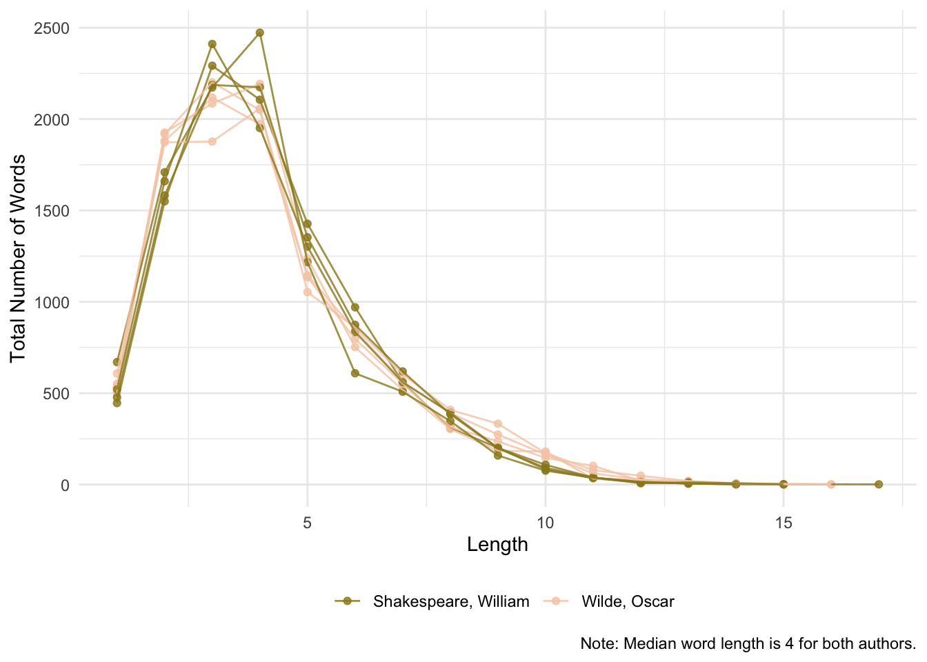
Are there any differences? What can we conclude from the evidence? What are the limitations of this approach? Are there alternative approaches to study what Mendenhall was getting at?
1.5 Exercise (Optional)
- Extend the current analysis to other authors or to more works from the same author.
- Are there better ways to compare the distribution of word length? Are there changes across time? Are there differences between different types of works (e.g., fiction vs. non-fiction, prose vs. poetry)?
1.6 Final Words
As will be often the case, we won’t be able to cover every single feature that the different packages have to offer, or how some objects that we create look like, or what else we can do with them. My advise is that you go home and explore the code in detail. Try applying the code to a different corpus and come next class with questions (or just show off what you were able to do).