5 Week 5: Scaling Techniques and Topic Modeling

Slides

6 Scaling Techniques and Topic Modeling (link or in Perusall)

5.1 Setup

As always, we first load the packages that we’ll be using:

# devtools::install_github("conjugateprior/austin")
library(austin) # just for those sweet wordscores
library(tidyverse) # for wrangling data
library(tidylog) # to know what we are wrangling
library(tidytext) # for 'tidy' manipulation of text data
library(quanteda) # tokenization power house
library(quanteda.textmodels)
library(stm) # run structural topic models
library(wesanderson) # to prettify

5.2 Wordscores

Laver et al. (2003) propose a supervised scaling technique called wordscores. We learned about the intuition in this weeks lecture. We will now replicate Table 1 from Laver and Benoit (2003) using the austin package. The package includes some sample data we will be using:

data(lbg)

Let’s keep only the reference documents:

ref <- getdocs(lbg, 1:5)
ref

##      docs
## words  R1  R2  R3  R4  R5
##    A    2   0   0   0   0
##    B    3   0   0   0   0
##    C   10   0   0   0   0
##    D   22   0   0   0   0
##    E   45   0   0   0   0
##    F   78   2   0   0   0
##    G  115   3   0   0   0
##    H  146  10   0   0   0
##    I  158  22   0   0   0
##    J  146  45   0   0   0
##    K  115  78   2   0   0
##    L   78 115   3   0   0
##    M   45 146  10   0   0
##    N   22 158  22   0   0
##    O   10 146  45   0   0
##    P    3 115  78   2   0
##    Q    2  78 115   3   0
##    R    0  45 146  10   0
##    S    0  22 158  22   0
##    T    0  10 146  45   0
##    U    0   3 115  78   2
##    V    0   2  78 115   3
##    W    0   0  45 146  10
##    X    0   0  22 158  22
##    Y    0   0  10 146  45
##    Z    0   0   3 115  78
##    ZA   0   0   2  78 115
##    ZB   0   0   0  45 146
##    ZC   0   0   0  22 158
##    ZD   0   0   0  10 146
##    ZE   0   0   0   3 115
##    ZF   0   0   0   2  78
##    ZG   0   0   0   0  45
##    ZH   0   0   0   0  22
##    ZI   0   0   0   0  10
##    ZJ   0   0   0   0   3
##    ZK   0   0   0   0   2

This is the same matrix from Figure 1, where we have a count for the count of each word (in this case, letters) by reference document (the documents that have been previously labelled). We can give scores A_scores to each reference text to place them in a ideological scale (or whatever scale we want). We then estimate the wordscores for each word.

# We do this in the order of the reference texts:
A_score <- c(-1.5,-0.75,0,0.75,1.5)
ws <- classic.wordscores(ref, scores=A_score)
ws$pi

##         Score
## A  -1.5000000
## B  -1.5000000
## C  -1.5000000
## D  -1.5000000
## E  -1.5000000
## F  -1.4812500
## G  -1.4809322
## H  -1.4519231
## I  -1.4083333
## J  -1.3232984
## K  -1.1846154
## L  -1.0369898
## M  -0.8805970
## N  -0.7500000
## O  -0.6194030
## P  -0.4507576
## Q  -0.2992424
## R  -0.1305970
## S   0.0000000
## T   0.1305970
## U   0.2992424
## V   0.4507576
## W   0.6194030
## X   0.7500000
## Y   0.8805970
## Z   1.0369898
## ZA  1.1846154
## ZB  1.3232984
## ZC  1.4083333
## ZD  1.4519231
## ZE  1.4809322
## ZF  1.4812500
## ZG  1.5000000
## ZH  1.5000000
## ZI  1.5000000
## ZJ  1.5000000
## ZK  1.5000000

Now we get the virgin text and predict the textscore by estimating the average of the weighted wordscores for the virgin document:

vir <- getdocs(lbg, 'V1')
vir

##      docs
## words  V1
##    A    0
##    B    0
##    C    0
##    D    0
##    E    0
##    F    0
##    G    0
##    H    2
##    I    3
##    J   10
##    K   22
##    L   45
##    M   78
##    N  115
##    O  146
##    P  158
##    Q  146
##    R  115
##    S   78
##    T   45
##    U   22
##    V   10
##    W    3
##    X    2
##    Y    0
##    Z    0
##    ZA   0
##    ZB   0
##    ZC   0
##    ZD   0
##    ZE   0
##    ZF   0
##    ZG   0
##    ZH   0
##    ZI   0
##    ZJ   0
##    ZK   0

# predict textscores for the virgin documents
predict(ws, newdata=vir)

## 37 of 37 words (100%) are scorable
## 
##     Score Std. Err. Rescaled  Lower  Upper
## V1 -0.448    0.0119   -0.448 -0.459 -0.437

Cool.

5.3 Wordfish

Slapin and Proksch (2008) propose an unsupervised scaling model that places texts in a one-dimensional scale. The underlying assumption is that in

\[w_{ik} ∼ Poisson(\lambda _{ik})\] \[\lambda_{ik} = exp(α_i +ψ_k +β_k ×θ_i)\]

\(\lambda_{ik}\) is generated by \(α_i\) (the “loquaciousness” of politician \(i\) or document fixed-effects), \(ψ_k\) (the frequency of word k), \(β_k\) (the discrimination parameter of word \(k\)) and, most importantly, \(θ_i\) (the politician’s ideological position). Let’s believe for a moment that the peer-review system works and use the textmodel_wordfish() function to estimate the ideological positions of U.S. Presidents using their inaugural speeches.

us_pres <- readxl::read_xlsx(path = "data/inaugTexts.xlsx")
head(us_pres)

## # A tibble: 6 × 4
##   inaugSpeech                                               Year President party
##   <chr>                                                    <dbl> <chr>     <chr>
## 1 "My Countrymen, It a relief to feel that no heart but m…  1853 Pierce    Demo…
## 2 "Fellow citizens, I appear before you this day to take …  1857 Buchanan  Demo…
## 3 "Fellow-Citizens of the United States: In compliance wi…  1861 Lincoln   Repu…
## 4 "Fellow-Countrymen:\r\n\r\nAt this second appearing to …  1865 Lincoln   Repu…
## 5 "Citizens of the United States:\r\n\r\nYour suffrages h…  1869 Grant     Repu…
## 6 "Fellow-Citizens:\r\n\r\nUnder Providence I have been c…  1873 Grant     Repu…

The text is pretty clean, so we can change it into a corpus object and then a dfm and apply textmodel_wordfish():

corpus_us_pres <- corpus(us_pres,
                     text_field = "inaugSpeech",
                     unique_docnames = TRUE)

summary(corpus_us_pres)

## Corpus consisting of 41 documents, showing 41 documents:
## 
##    Text Types Tokens Sentences Year    President      party
##   text1  1164   3631       104 1853       Pierce   Democrat
##   text2   944   3080        89 1857     Buchanan   Democrat
##   text3  1074   3992       135 1861      Lincoln Republican
##   text4   359    774        26 1865      Lincoln Republican
##   text5   484   1223        40 1869        Grant Republican
##   text6   551   1469        43 1873        Grant Republican
##   text7   830   2698        59 1877        Hayes Republican
##   text8  1020   3206       111 1881     Garfield Republican
##   text9   675   1812        44 1885    Cleveland   Democrat
##  text10  1351   4720       157 1889     Harrison Republican
##  text11   821   2125        58 1893    Cleveland   Democrat
##  text12  1231   4345       130 1897     McKinley Republican
##  text13   854   2437       100 1901     McKinley Republican
##  text14   404   1079        33 1905  T Roosevelt Republican
##  text15  1437   5821       158 1909         Taft Republican
##  text16   658   1882        68 1913       Wilson   Democrat
##  text17   548   1648        59 1917       Wilson   Democrat
##  text18  1168   3717       148 1921      Harding Republican
##  text19  1220   4440       196 1925     Coolidge Republican
##  text20  1089   3855       158 1929       Hoover Republican
##  text21   742   2052        85 1933 FD Roosevelt   Democrat
##  text22   724   1981        96 1937 FD Roosevelt   Democrat
##  text23   525   1494        68 1941 FD Roosevelt   Democrat
##  text24   274    619        27 1945 FD Roosevelt   Democrat
##  text25   780   2495       116 1949       Truman   Democrat
##  text26   899   2729       119 1953   Eisenhower Republican
##  text27   620   1883        92 1957   Eisenhower Republican
##  text28   565   1516        52 1961      Kennedy   Democrat
##  text29   567   1697        93 1965      Johnson   Democrat
##  text30   742   2395       103 1969        Nixon Republican
##  text31   543   1978        68 1973        Nixon Republican
##  text32   527   1363        52 1977       Carter   Democrat
##  text33   901   2771       129 1981       Reagan Republican
##  text34   924   2897       124 1985       Reagan Republican
##  text35   794   2666       141 1989         Bush Republican
##  text36   642   1833        81 1993      Clinton   Democrat
##  text37   772   2423       111 1997      Clinton   Democrat
##  text38   620   1804        97 2001         Bush Republican
##  text39   773   2321       100 2005         Bush Republican
##  text40   937   2667       110 2009        Obama   Democrat
##  text41   814   2317        88 2013        Obama   Democrat

# We do the whole tokenization sequence
toks_us_pres <- tokens(corpus_us_pres,
                   remove_numbers = TRUE, # Thinks about this
                   remove_punct = TRUE, # Remove punctuation!
                   remove_url = TRUE) # Might be helpful

toks_us_pres <- tokens_remove(toks_us_pres,
                              # Should we though? See Denny and Spirling (2018)
                              c(stopwords(language = "en")),
                              padding = F)

toks_us_pres <- tokens_wordstem(toks_us_pres, language = "en")

dfm_us_pres <- dfm(toks_us_pres)

wfish_us_pres <- textmodel_wordfish(dfm_us_pres, dir = c(28,30)) #Does not really matter what the starting values are, they just serve as anchors for the relative position of the rest of the texts. In this case, I chose Kennedy and Nixon.  
summary(wfish_us_pres)

## 
## Call:
## textmodel_wordfish.dfm(x = dfm_us_pres, dir = c(28, 30))
## 
## Estimated Document Positions:
##           theta      se
## text1  -0.95629 0.03619
## text2  -1.27077 0.03413
## text3  -1.40878 0.02863
## text4  -0.37189 0.08907
## text5  -1.19374 0.05617
## text6  -0.98770 0.05747
## text7  -1.25058 0.03681
## text8  -1.15827 0.03506
## text9  -1.06959 0.04866
## text10 -1.37028 0.02601
## text11 -1.09563 0.04336
## text12 -1.36432 0.02716
## text13 -0.96921 0.04392
## text14  0.14969 0.07992
## text15 -1.67350 0.01837
## text16  0.04362 0.05968
## text17 -0.14872 0.06481
## text18 -0.23053 0.04050
## text19 -0.64321 0.03619
## text20 -0.81689 0.03636
## text21 -0.26532 0.05470
## text22  0.26579 0.05564
## text23  0.56628 0.06543
## text24  0.82820 0.09574
## text25  0.09676 0.04999
## text26  0.37480 0.04777
## text27  0.60678 0.05655
## text28  0.92039 0.05651
## text29  0.95967 0.05604
## text30  1.42421 0.03773
## text31  0.93162 0.05098
## text32  0.87564 0.06215
## text33  1.13335 0.04084
## text34  1.19832 0.03745
## text35  1.26112 0.03960
## text36  1.38125 0.04374
## text37  1.37962 0.03680
## text38  0.86932 0.05416
## text39  0.74023 0.04862
## text40  1.18811 0.03946
## text41  1.05044 0.04446
## 
## Estimated Feature Scores:
##      countrymen  relief    feel   heart    can   know  person  regret   bitter
## beta    -0.5490 -0.9578 -0.4909 0.80654 0.1395 0.9422 -0.1117 -0.2531  0.00357
## psi     -0.5455 -1.8438 -0.3950 0.08677 2.1155 0.6955 -0.1544 -2.8008 -2.01944
##       sorrow    born   posit suitabl  other    rather   desir circumst   call
## beta  0.5176  0.7626 -0.9823  -4.120 0.3938  0.005296 -0.6213  -0.6355 0.3744
## psi  -2.0333 -0.8259 -1.2129  -6.134 0.1718 -0.591942 -0.5404  -1.3620 0.5610
##         limit    period presid destini   republ    fill profound    sens
## beta -0.07365 -0.004602 0.4897  0.2596 -0.27095  0.6832 -0.05067 -0.1156
## psi  -0.02462 -1.040467 0.4726 -0.2598  0.08116 -1.6845 -1.52213 -0.2337
##      respons     noth    like  shrink
## beta  0.2263 -0.08437 0.01591  0.1689
## psi   0.8392 -0.25100 0.19881 -1.7082

Let’s see if this made any sense. Since we have the party of the president, we should see the Republican cluster together and apart from Democrats (or something):

# Get predictions:
wfish_preds <- predict(wfish_us_pres, interval = "confidence")

# Tidy everything up:
posi_us_pres <- data.frame(docvars(corpus_us_pres),
                      wfish_preds$fit) %>%
  arrange(fit)

# Plot
posi_us_pres %>%
  ggplot(aes(x = fit, y = reorder(President,fit), xmin = lwr, xmax = upr, color = party)) +
  geom_point(alpha = 0.8) +
  geom_errorbarh(height = 0) +
  labs(x = "Position", y = "", color = "Party") +
  scale_color_manual(values = wes_palette("BottleRocket2")) +
  theme_minimal() +
  ggtitle("Estimated Positions")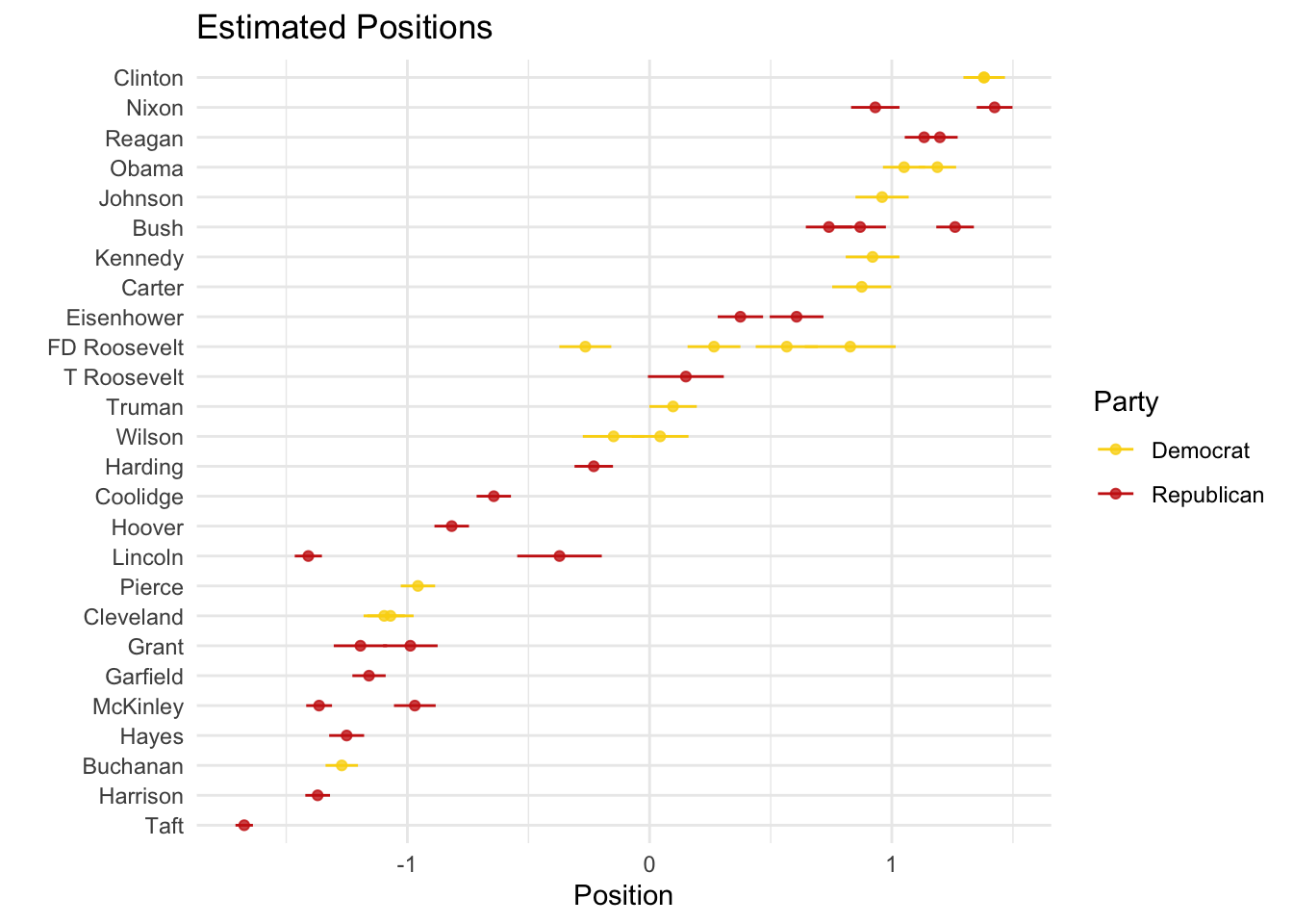

Two things to note. First, the direction of the scale is a theoretically-based decision that the researcher has to make (not the algorithm). In our case, based on the results, we could say that the positive values are more left-leaning and the negative values are more right-leaning. We can switch that (for visualization purposes) just by multiplying by -1:

# Plot inverse
posi_us_pres %>%
  ggplot(aes(x = -fit, y = reorder(President,fit), xmin = -lwr, xmax = -upr, color = party)) +
  geom_point(alpha = 0.8) +
  geom_errorbarh(height = 0) +
  labs(x = "Position", y = "", color = "Party") +
  scale_color_manual(values = wes_palette("BottleRocket2")) +
  theme_minimal() +
  ggtitle("Estimated Positions")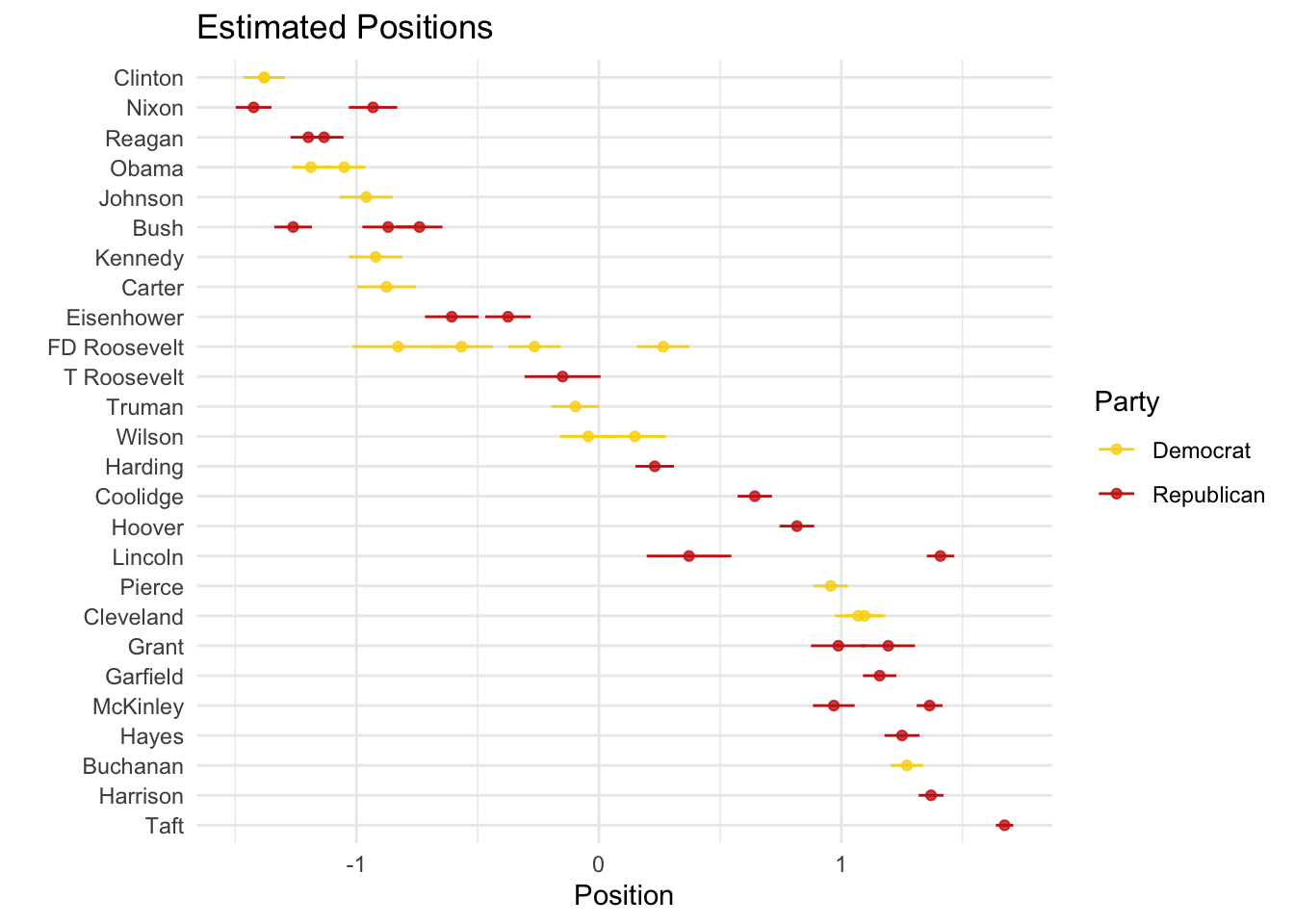

Second, there seems to be a mismatch between our theoretical expectations and our empirical observations. We would assume that Republicans (Democrats) will talk similarly to other Republicans (Democrats) and different from Democrats (Republicans). However, this is not the case. What could be happening?

One answer could be that language changes over time or that issues change over time or that what it meant to be a Democrat and Republican changed over time, and that change is being picked up by the model:

# Plot time
posi_us_pres %>%
  ggplot(aes(y = -fit, x = Year, ymin = -lwr, ymax = -upr, color = party)) +
  geom_point(alpha = 0.8) +
  geom_errorbar() +
  labs(x = "Year", y = "Position", color = "Party") +
  scale_color_manual(values = wes_palette("BottleRocket2")) +
  theme_minimal() +
  ggtitle("Estimated Positions")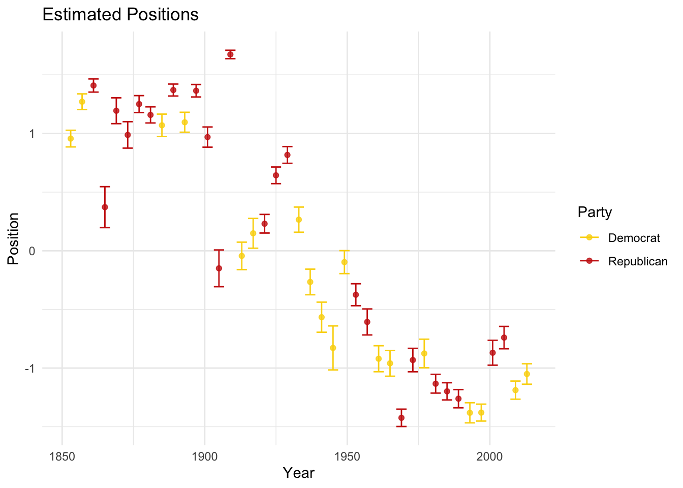

That seems to be one possible explanation. The other could be that the pre-processing steps substantively modified the texts (see Denny and Spirling 2018). We can estimate the model again using a different pre-processed text:

# Tokenization only removing punctuation
toks_us_pres2 <- tokens(corpus_us_pres,
                   remove_punct = TRUE) 

dfm_us_pres2 <- dfm(toks_us_pres2)
wfish_us_pres <- textmodel_wordfish(dfm_us_pres2, dir = c(28,30))  

# Get predictions:
wfish_preds <- predict(wfish_us_pres, interval = "confidence")

# Tidy everything up:
posi_us_pres <- data.frame(docvars(corpus_us_pres),
                      wfish_preds$fit) %>%
  arrange(fit)

# Plot
posi_us_pres %>%
  ggplot(aes(x = -fit, y = reorder(President,fit), xmin = -lwr, xmax = -upr, color = party)) +
  geom_point(alpha = 0.8) +
  geom_errorbarh(height = 0) +
  labs(x = "Position", y = "", color = "Party") +
  scale_color_manual(values = wes_palette("BottleRocket2")) +
  theme_minimal() +
  ggtitle("Estimated Positions (No Pre-Processing")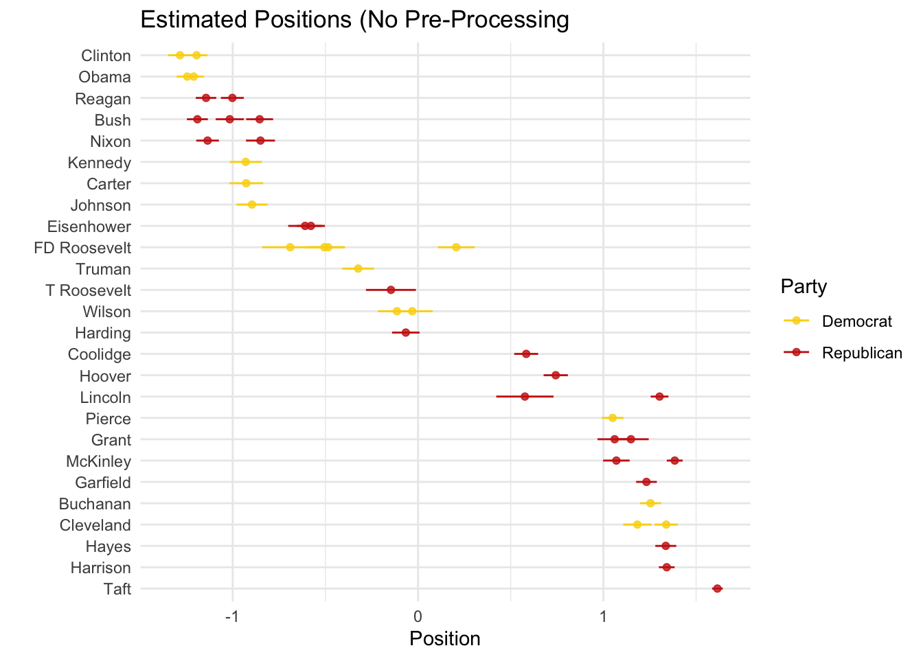

At the very least, the within president differences in estimates have narrowed, but time seems to still be the best predictor:

# Plot time
posi_us_pres %>%
  ggplot(aes(y = -fit, x = Year, ymin = -lwr, ymax = -upr, color = party)) +
  geom_point(alpha = 0.8) +
  geom_errorbar() +
  labs(x = "Year", y = "Position", color = "Party") +
  scale_color_manual(values = wes_palette("BottleRocket2")) +
  theme_minimal() +
  ggtitle("Estimated Positions")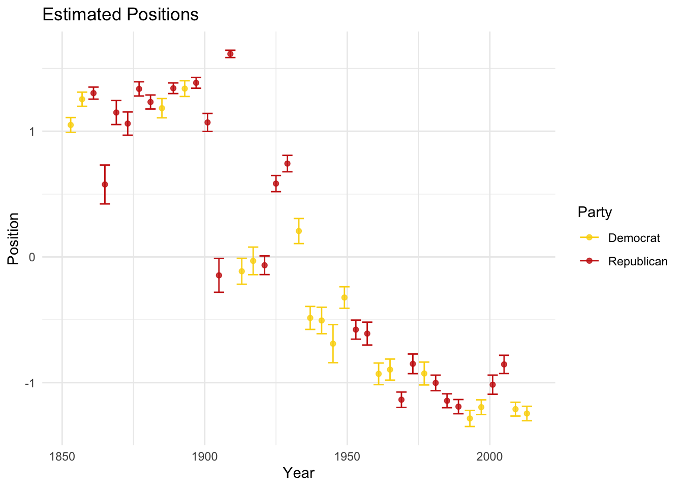

If time is the main predictor, then maybe we need to think about periods of time that are comparable for both parties (e.g., after the Civil Rights Act).

5.4 Structural Topic Models

STM provides two ways to include contextual information to “guide” the estimation of the model. First, topic prevalence can vary by metadata (e.g. Republicans talk about military issues more than Democrats). Second, topic content can vary by metadata (e.g. Republicans talk about military issues differently from Democrats).

We can run STM using the stm package. The stm package includes the complete workflow (i.e. from raw text to figures), and if you are planning to use it in the future I highly encourage you to check this and this and this and this. stm() takes our dfm and produces topics. If we do not specify any prevalence terms, then it will estimate an LDA. Since this is a Bayesian approach, it is recommended you set a seed value for future replication. We also need to set \(K\) number of topics. How many topics are the right number of topics? There is no good number. Too many pre-specified topics and the categories might be meaningless. Too few, and you might be piling together two or more topics. Note that changes to a) the number of topics, b) the prevalence term, c) the omitted words, d) the seed value, can (greatly) change the outcome. Here is where validation becomes crucial (for a review see Wilkerson and Casas 2017).

Using our presidential speeches data, I will use stm to estimate the topics surrounding the inaugural addresses. As my prevalence term, I add the party of the speaker. I set my number of topics at 10 (but with a corpus this big I should probably set it at ~30 and work my way up from there).

stm_us_pres <- stm(dfm_us_pres, K = 10, seed = 1984,
                   prevalence = ~party,
                   init.type = "Spectral")

## Beginning Spectral Initialization 
##   Calculating the gram matrix...
##   Finding anchor words...
##      ..........
##   Recovering initialization...
##      ..............................................
## Initialization complete.
## .........................................
## Completed E-Step (0 seconds). 
## Completed M-Step. 
## Completing Iteration 1 (approx. per word bound = -7.071) 
## .........................................
## Completed E-Step (0 seconds). 
## Completed M-Step. 
## Completing Iteration 2 (approx. per word bound = -6.881, relative change = 2.689e-02) 
## .........................................
## Completed E-Step (0 seconds). 
## Completed M-Step. 
## Completing Iteration 3 (approx. per word bound = -6.819, relative change = 8.961e-03) 
## .........................................
## Completed E-Step (0 seconds). 
## Completed M-Step. 
## Completing Iteration 4 (approx. per word bound = -6.790, relative change = 4.253e-03) 
## .........................................
## Completed E-Step (0 seconds). 
## Completed M-Step. 
## Completing Iteration 5 (approx. per word bound = -6.780, relative change = 1.521e-03) 
## Topic 1: us, new, world, nation, let 
##  Topic 2: new, can, us, nation, work 
##  Topic 3: constitut, state, union, can, law 
##  Topic 4: nation, must, us, peopl, can 
##  Topic 5: govern, peopl, upon, state, law 
##  Topic 6: nation, freedom, america, govern, peopl 
##  Topic 7: us, america, must, nation, american 
##  Topic 8: upon, nation, govern, peopl, shall 
##  Topic 9: world, nation, peopl, peac, can 
##  Topic 10: us, nation, govern, must, peopl 
## .........................................
## Completed E-Step (0 seconds). 
## Completed M-Step. 
## Completing Iteration 6 (approx. per word bound = -6.775, relative change = 6.929e-04) 
## .........................................
## Completed E-Step (0 seconds). 
## Completed M-Step. 
## Completing Iteration 7 (approx. per word bound = -6.771, relative change = 5.320e-04) 
## .........................................
## Completed E-Step (0 seconds). 
## Completed M-Step. 
## Completing Iteration 8 (approx. per word bound = -6.768, relative change = 5.267e-04) 
## .........................................
## Completed E-Step (0 seconds). 
## Completed M-Step. 
## Completing Iteration 9 (approx. per word bound = -6.765, relative change = 4.328e-04) 
## .........................................
## Completed E-Step (0 seconds). 
## Completed M-Step. 
## Completing Iteration 10 (approx. per word bound = -6.763, relative change = 3.022e-04) 
## Topic 1: us, new, world, let, nation 
##  Topic 2: us, new, can, nation, work 
##  Topic 3: constitut, state, union, can, shall 
##  Topic 4: nation, must, peopl, us, world 
##  Topic 5: govern, peopl, upon, law, state 
##  Topic 6: nation, freedom, america, peopl, govern 
##  Topic 7: us, america, must, nation, american 
##  Topic 8: upon, nation, govern, peopl, can 
##  Topic 9: nation, world, peopl, peac, can 
##  Topic 10: us, govern, nation, peopl, must 
## .........................................
## Completed E-Step (0 seconds). 
## Completed M-Step. 
## Completing Iteration 11 (approx. per word bound = -6.762, relative change = 2.094e-04) 
## .........................................
## Completed E-Step (0 seconds). 
## Completed M-Step. 
## Completing Iteration 12 (approx. per word bound = -6.760, relative change = 1.745e-04) 
## .........................................
## Completed E-Step (0 seconds). 
## Completed M-Step. 
## Completing Iteration 13 (approx. per word bound = -6.759, relative change = 1.485e-04) 
## .........................................
## Completed E-Step (0 seconds). 
## Completed M-Step. 
## Completing Iteration 14 (approx. per word bound = -6.759, relative change = 1.147e-04) 
## .........................................
## Completed E-Step (0 seconds). 
## Completed M-Step. 
## Completing Iteration 15 (approx. per word bound = -6.758, relative change = 1.018e-04) 
## Topic 1: us, new, let, world, nation 
##  Topic 2: us, new, can, nation, work 
##  Topic 3: constitut, state, union, can, shall 
##  Topic 4: nation, must, peopl, us, world 
##  Topic 5: govern, peopl, upon, law, state 
##  Topic 6: nation, freedom, america, peopl, govern 
##  Topic 7: us, america, must, nation, american 
##  Topic 8: upon, nation, govern, peopl, can 
##  Topic 9: nation, peopl, world, can, peac 
##  Topic 10: us, govern, nation, peopl, must 
## .........................................
## Completed E-Step (0 seconds). 
## Completed M-Step. 
## Completing Iteration 16 (approx. per word bound = -6.757, relative change = 9.728e-05) 
## .........................................
## Completed E-Step (0 seconds). 
## Completed M-Step. 
## Completing Iteration 17 (approx. per word bound = -6.757, relative change = 8.328e-05) 
## .........................................
## Completed E-Step (0 seconds). 
## Completed M-Step. 
## Completing Iteration 18 (approx. per word bound = -6.756, relative change = 7.150e-05) 
## .........................................
## Completed E-Step (0 seconds). 
## Completed M-Step. 
## Completing Iteration 19 (approx. per word bound = -6.756, relative change = 5.364e-05) 
## .........................................
## Completed E-Step (0 seconds). 
## Completed M-Step. 
## Completing Iteration 20 (approx. per word bound = -6.756, relative change = 3.903e-05) 
## Topic 1: us, new, let, world, nation 
##  Topic 2: us, new, can, nation, work 
##  Topic 3: constitut, state, govern, shall, union 
##  Topic 4: nation, must, peopl, us, world 
##  Topic 5: govern, peopl, upon, law, state 
##  Topic 6: nation, freedom, america, peopl, govern 
##  Topic 7: us, america, must, nation, american 
##  Topic 8: upon, nation, govern, peopl, can 
##  Topic 9: nation, peopl, world, can, peac 
##  Topic 10: us, govern, nation, peopl, must 
## .........................................
## Completed E-Step (0 seconds). 
## Completed M-Step. 
## Completing Iteration 21 (approx. per word bound = -6.755, relative change = 3.678e-05) 
## .........................................
## Completed E-Step (0 seconds). 
## Completed M-Step. 
## Completing Iteration 22 (approx. per word bound = -6.755, relative change = 3.378e-05) 
## .........................................
## Completed E-Step (0 seconds). 
## Completed M-Step. 
## Completing Iteration 23 (approx. per word bound = -6.755, relative change = 3.008e-05) 
## .........................................
## Completed E-Step (0 seconds). 
## Completed M-Step. 
## Completing Iteration 24 (approx. per word bound = -6.755, relative change = 3.311e-05) 
## .........................................
## Completed E-Step (0 seconds). 
## Completed M-Step. 
## Completing Iteration 25 (approx. per word bound = -6.754, relative change = 3.247e-05) 
## Topic 1: us, new, let, world, nation 
##  Topic 2: us, new, can, nation, work 
##  Topic 3: constitut, state, govern, peopl, shall 
##  Topic 4: nation, must, peopl, us, world 
##  Topic 5: govern, peopl, upon, law, state 
##  Topic 6: nation, freedom, america, govern, peopl 
##  Topic 7: us, must, america, nation, american 
##  Topic 8: upon, nation, govern, peopl, can 
##  Topic 9: nation, peopl, world, can, peac 
##  Topic 10: us, govern, nation, peopl, must 
## .........................................
## Completed E-Step (0 seconds). 
## Completed M-Step. 
## Completing Iteration 26 (approx. per word bound = -6.754, relative change = 2.886e-05) 
## .........................................
## Completed E-Step (0 seconds). 
## Completed M-Step. 
## Completing Iteration 27 (approx. per word bound = -6.754, relative change = 2.778e-05) 
## .........................................
## Completed E-Step (0 seconds). 
## Completed M-Step. 
## Completing Iteration 28 (approx. per word bound = -6.754, relative change = 2.814e-05) 
## .........................................
## Completed E-Step (0 seconds). 
## Completed M-Step. 
## Completing Iteration 29 (approx. per word bound = -6.754, relative change = 4.342e-05) 
## .........................................
## Completed E-Step (0 seconds). 
## Completed M-Step. 
## Completing Iteration 30 (approx. per word bound = -6.753, relative change = 2.111e-05) 
## Topic 1: us, new, let, nation, world 
##  Topic 2: us, new, can, nation, work 
##  Topic 3: constitut, state, govern, peopl, shall 
##  Topic 4: nation, peopl, must, us, world 
##  Topic 5: govern, peopl, upon, law, state 
##  Topic 6: nation, freedom, america, govern, peopl 
##  Topic 7: us, must, america, nation, american 
##  Topic 8: upon, nation, govern, peopl, can 
##  Topic 9: nation, peopl, world, can, peac 
##  Topic 10: us, govern, nation, peopl, world 
## .........................................
## Completed E-Step (0 seconds). 
## Completed M-Step. 
## Completing Iteration 31 (approx. per word bound = -6.753, relative change = 1.621e-05) 
## .........................................
## Completed E-Step (0 seconds). 
## Completed M-Step. 
## Completing Iteration 32 (approx. per word bound = -6.753, relative change = 1.678e-05) 
## .........................................
## Completed E-Step (0 seconds). 
## Completed M-Step. 
## Completing Iteration 33 (approx. per word bound = -6.753, relative change = 1.686e-05) 
## .........................................
## Completed E-Step (0 seconds). 
## Completed M-Step. 
## Completing Iteration 34 (approx. per word bound = -6.753, relative change = 1.705e-05) 
## .........................................
## Completed E-Step (0 seconds). 
## Completed M-Step. 
## Completing Iteration 35 (approx. per word bound = -6.753, relative change = 1.793e-05) 
## Topic 1: us, new, let, nation, world 
##  Topic 2: us, new, can, nation, work 
##  Topic 3: constitut, state, govern, peopl, shall 
##  Topic 4: nation, peopl, must, us, world 
##  Topic 5: govern, peopl, upon, law, state 
##  Topic 6: nation, freedom, america, govern, peopl 
##  Topic 7: us, must, america, nation, american 
##  Topic 8: upon, nation, govern, peopl, can 
##  Topic 9: nation, peopl, world, can, peac 
##  Topic 10: us, govern, nation, peopl, world 
## .........................................
## Completed E-Step (0 seconds). 
## Completed M-Step. 
## Completing Iteration 36 (approx. per word bound = -6.753, relative change = 2.033e-05) 
## .........................................
## Completed E-Step (0 seconds). 
## Completed M-Step. 
## Completing Iteration 37 (approx. per word bound = -6.753, relative change = 2.216e-05) 
## .........................................
## Completed E-Step (0 seconds). 
## Completed M-Step. 
## Completing Iteration 38 (approx. per word bound = -6.752, relative change = 1.878e-05) 
## .........................................
## Completed E-Step (0 seconds). 
## Completed M-Step. 
## Completing Iteration 39 (approx. per word bound = -6.752, relative change = 1.591e-05) 
## .........................................
## Completed E-Step (0 seconds). 
## Completed M-Step. 
## Completing Iteration 40 (approx. per word bound = -6.752, relative change = 1.384e-05) 
## Topic 1: us, new, let, nation, world 
##  Topic 2: us, new, can, nation, work 
##  Topic 3: constitut, state, govern, peopl, shall 
##  Topic 4: nation, peopl, must, us, world 
##  Topic 5: govern, peopl, upon, law, state 
##  Topic 6: nation, freedom, america, govern, peopl 
##  Topic 7: us, must, america, nation, american 
##  Topic 8: upon, nation, govern, peopl, can 
##  Topic 9: nation, peopl, world, can, peac 
##  Topic 10: us, govern, nation, peopl, world 
## .........................................
## Completed E-Step (0 seconds). 
## Completed M-Step. 
## Completing Iteration 41 (approx. per word bound = -6.752, relative change = 1.337e-05) 
## .........................................
## Completed E-Step (0 seconds). 
## Completed M-Step. 
## Completing Iteration 42 (approx. per word bound = -6.752, relative change = 1.381e-05) 
## .........................................
## Completed E-Step (0 seconds). 
## Completed M-Step. 
## Completing Iteration 43 (approx. per word bound = -6.752, relative change = 1.388e-05) 
## .........................................
## Completed E-Step (0 seconds). 
## Completed M-Step. 
## Completing Iteration 44 (approx. per word bound = -6.752, relative change = 1.720e-05) 
## .........................................
## Completed E-Step (0 seconds). 
## Completed M-Step. 
## Completing Iteration 45 (approx. per word bound = -6.752, relative change = 1.363e-05) 
## Topic 1: us, new, let, nation, world 
##  Topic 2: us, new, can, nation, work 
##  Topic 3: constitut, state, govern, peopl, shall 
##  Topic 4: nation, peopl, must, us, world 
##  Topic 5: govern, peopl, upon, law, state 
##  Topic 6: nation, freedom, america, peopl, govern 
##  Topic 7: us, must, america, nation, american 
##  Topic 8: upon, nation, govern, peopl, can 
##  Topic 9: nation, peopl, world, can, peac 
##  Topic 10: us, govern, nation, peopl, world 
## .........................................
## Completed E-Step (0 seconds). 
## Completed M-Step. 
## Completing Iteration 46 (approx. per word bound = -6.752, relative change = 1.725e-05) 
## .........................................
## Completed E-Step (0 seconds). 
## Completed M-Step. 
## Completing Iteration 47 (approx. per word bound = -6.752, relative change = 1.410e-05) 
## .........................................
## Completed E-Step (0 seconds). 
## Completed M-Step. 
## Model Converged

The nice thing about the stm() function is that it allows us to see in “real-time” what is going on within the black box. We can summarize the process in the following way (this is similar to a collapsed Gibbs sampling, which the stm() function sort of uses):

Go through each document, and randomly assign each word in the document to one of the topics \(\displaystyle t\in k\).
Notice that this random assignment already gives both topic representations of all the documents and word distributions of all the topics (albeit not very good ones).
So to improve on them, for each document \(\displaystyle W\) do the following:

3.1 Go through each word \(\displaystyle w\) in \(\displaystyle W\)

3.1.1 And for each topic \(\displaystyle t\), compute two things:

3.1.1.1 \(\displaystyle p(t|W)\) = the proportion of words in document \(\displaystyle W\) that are currently assigned to topic \(\displaystyle t\), and

3.1.1.2 \(\displaystyle p(w|t)\) = the proportion of assignments to topic \(\displaystyle t\) over all documents that come from this word \(\displaystyle w\). Reassign \(\displaystyle w\) a new topic, where we choose topic \(\displaystyle t\) with probability \(\displaystyle p(t|W)*p(w|t)\). It is worth noting that according to our generative model, this is essentially the probability that topic \(\displaystyle t\) generated word \(\displaystyle w\), so it makes sense that we resample the current word’s topic with this probability. (Also, I’m glossing over a couple of things here, in particular the use of priors/pseudocounts in these probabilities.)

3.1.1.3 In other words, in this step, we’re assuming that all topic assignments except for the current word in question are correct, and then updating the assignment of the current word using our model of how documents are generated.

After repeating the previous step a large number of times, you’ll eventually reach a roughly steady state where your assignments are pretty good. So use these assignments to estimate the topic mixtures of each document (by counting the proportion of words assigned to each topic within that document) and the words associated with each topic (by counting the proportion of words assigned to each topic overall).

(This explanation was taken from here). Let’s explore the topics produced:

labelTopics(stm_us_pres)

## Topic 1 Top Words:
##       Highest Prob: us, new, let, nation, world, can, america 
##       FREX: let, centuri, togeth, dream, new, promis, weak 
##       Lift: 200th, 20th, micah, rhetor, 18th, 19th, accident 
##       Score: role, dream, abroad, third, explor, shape, proud 
## Topic 2 Top Words:
##       Highest Prob: us, new, can, nation, work, world, great 
##       FREX: friend, mr, thing, breez, word, blow, fact 
##       Lift: breez, crucial, addict, alloc, assistanc, bacteria, bicentenni 
##       Score: breez, crucial, blow, page, manger, thank, sometim 
## Topic 3 Top Words:
##       Highest Prob: constitut, state, govern, peopl, shall, can, law 
##       FREX: case, constitut, slave, union, territori, slaveri, minor 
##       Lift: alleg, anarchi, besid, compulsori, constru, cover, dissatisfi 
##       Score: case, slaveri, territori, slave, invas, provis, fli 
## Topic 4 Top Words:
##       Highest Prob: nation, peopl, must, us, world, can, govern 
##       FREX: activ, republ, task, confid, industri, inspir, normal 
##       Lift: abnorm, acclaim, aright, changer, comiti, frugal, gaze 
##       Score: normal, activ, amid, readjust, self-reli, relationship, unshaken 
## Topic 5 Top Words:
##       Highest Prob: govern, peopl, upon, law, state, countri, nation 
##       FREX: revenu, tariff, offic, appoint, busi, consider, proper 
##       Lift: ampli, antitrust, board, box, boycott, congression, dakota 
##       Score: revenu, legisl, enforc, polici, negro, interst, tariff 
## Topic 6 Top Words:
##       Highest Prob: nation, freedom, america, peopl, govern, know, democraci 
##       FREX: democraci, ideal, million, liberti, freedom, came, seen 
##       Lift: paint, >, aught, autocrat, baffl, baggag, beli 
##       Score: democraci, paint, million, magna, excus, seen, encount 
## Topic 7 Top Words:
##       Highest Prob: us, must, america, nation, american, world, peopl 
##       FREX: journey, stori, generat, storm, america, job, ideal 
##       Lift: afghanistan, aids, alongsid, anchor, anybodi, apathi, appalachia 
##       Score: stori, journey, job, capitol, storm, thank, drift 
## Topic 8 Top Words:
##       Highest Prob: upon, nation, govern, peopl, can, shall, great 
##       FREX: enforc, counsel, organ, island, thought, upon, integr 
##       Lift: cuba, eighteenth, adapt, aspect, creation, cuban, dilig 
##       Score: enforc, island, cuba, counsel, organ, eighteenth, adapt 
## Topic 9 Top Words:
##       Highest Prob: nation, peopl, world, can, peac, must, free 
##       FREX: resourc, contribut, repres, everywher, result, free, europ 
##       Lift: display, joint, likewis, mockeri, philosophi, array, barter 
##       Score: europ, philosophi, commun, contribut, precept, tax, program 
## Topic 10 Top Words:
##       Highest Prob: us, govern, nation, peopl, world, must, american 
##       FREX: weapon, tax, believ, hero, man, reduc, dream 
##       Lift: 50th, absent, adam, alamo, anger, ant, artilleri 
##       Score: weapon, hero, monument, nuclear, spend, tax, soviet

FREX weights words by their overall frequency and how exclusive they are to the topic. Lift weights words by dividing by their frequency in other topics, therefore giving higher weight to words that appear less frequently in other topics. Similar to Lift, Score divides the log frequency of the word in the topic by the log frequency of the word in other topics (Roberts et al. 2013). Bischof and Airoldi (2012) show the value of using FREX over the other measures.

You can use the plot() function to show the topics.

plot(stm_us_pres, type = "summary", labeltype = "frex") # or prob, lift score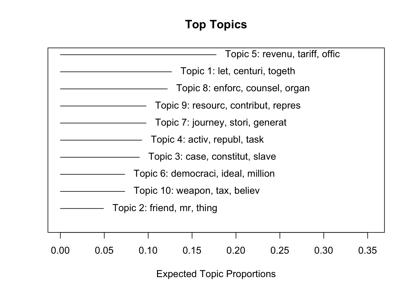

Topic 5 seems to be about the economy: revenue, tariffs, etc. Topic 3 about slavery adn the Civil War. If you want to see a sample of a specific topic:

findThoughts(stm_us_pres, texts = as.character(corpus_us_pres)[docnames(dfm_us_pres)], topics = 3)

That is a long speech.

We can (should/must) run some diagnostics. There are two qualities that were are looking for in our model: semantic coherence and exclusivity. Exclusivity is based on the FREX labeling matrix. Semantic coherence is a criterion developed by Mimno et al. (2011) and it maximizes when the most probable words in a given topic frequently co-occur together. Mimno et al. (2011) show that the metric correlates well with human judgement of topic quality. Yet, it is fairly easy to obtain high semantic coherence so it is important to see it in tandem with exclusivity. Let’s see how exclusive are the words in each topic:

dotchart(exclusivity(stm_us_pres), labels = 1:10)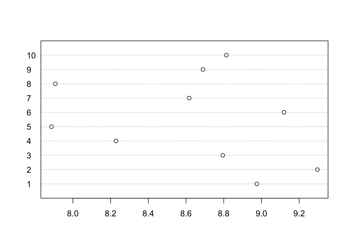

We can also see the semantic coherence of our topics –words a topic generates should co-occur often in the same document–:

dotchart(semanticCoherence(stm_us_pres,dfm_us_pres), labels = 1:10)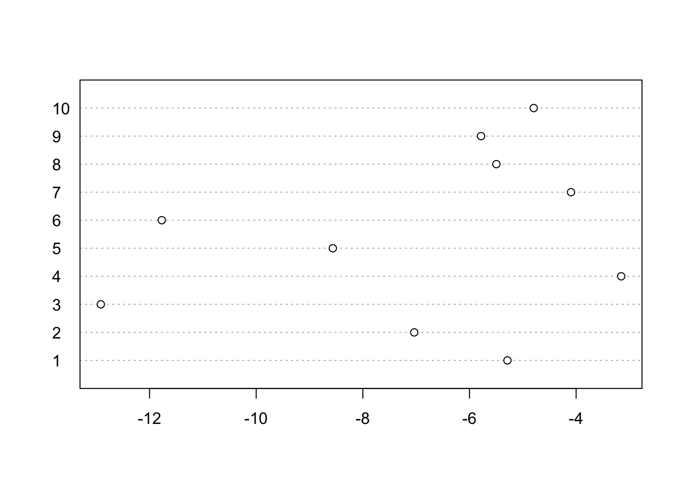

We can also see the overall quality of our topic model:

topicQuality(stm_us_pres,dfm_us_pres)

##  [1]  -5.287875  -7.035510 -12.913601  -3.154439  -8.562729 -11.770514
##  [7]  -4.095783  -5.495206  -5.782951  -4.794982
##  [1] 8.975188 9.296784 8.794789 8.229003 7.886663 9.119321 8.616780 7.907198
##  [9] 8.689432 8.813805

On their own, both metrics are not really useful (what do those numbers even mean?). They are useful when we are looking for the “optimal” number of topics.

stm_us_pres_10_15_20 <- manyTopics(dfm_us_pres,
                       prevalence = ~ party,
                       K = c(10,15,20), runs=2,
                       # max.em.its = 100, 
                       init.type = "Spectral") # It takes around 250 iterations for the model to converge. Depending on your computer, this can take a while.

We can now compare the performance of each model based on their semantic coherence and exclusivity. We are looking for high exclusivity and high coherence (top-right corner):

k_10 <- stm_us_pres_10_15_20$out[[1]] # k_10 is an stm object which can be explored and used like any other topic model. 
k_15 <- stm_us_pres_10_15_20$out[[2]]
k_20 <- stm_us_pres_10_15_20$out[[3]]

# I will just graph the 'quality' of each model:
topicQuality(k_10,dfm_us_pres)

##  [1]  -5.287875  -7.035510 -12.913601  -3.154439  -8.562729 -11.770514
##  [7]  -4.095783  -5.495206  -5.782951  -4.794982
##  [1] 8.975188 9.296784 8.794789 8.229003 7.886663 9.119321 8.616780 7.907198
##  [9] 8.689432 8.813805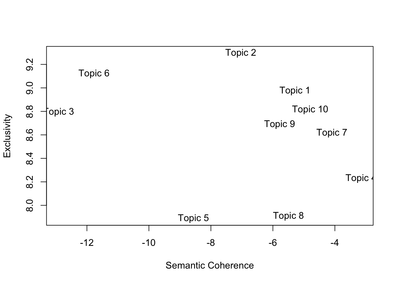

topicQuality(k_15,dfm_us_pres)

##  [1]  -8.282551 -10.661122  -9.146329  -6.243444 -10.002100 -11.315179
##  [7]  -3.107797  -4.907182  -5.059424  -4.905652  -7.864316 -13.149897
## [13]  -6.834348 -11.917696  -4.182962
##  [1] 9.225426 9.359212 9.252890 9.186251 9.037698 9.150213 8.615448 8.497762
##  [9] 8.545416 9.139213 8.183189 9.136856 8.467946 9.642172 8.453394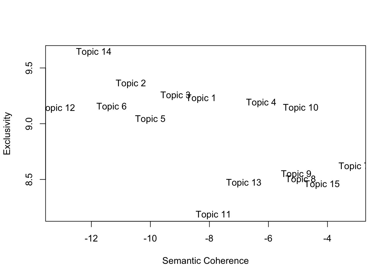

topicQuality(k_20,dfm_us_pres)

##  [1]  -8.136428 -22.245476 -21.390006  -6.602534 -11.543624 -10.272049
##  [7]  -3.923380  -5.506620  -7.188791 -12.486262 -10.086060 -13.443443
## [13] -15.978725 -12.256070 -10.137597 -11.231218  -6.177453  -4.358259
## [19]  -5.246579  -2.209688
##  [1] 9.489401 9.872037 9.761442 9.184861 9.370893 9.330946 9.019413 8.522081
##  [9] 8.633818 9.649097 8.307636 9.125968 8.957859 9.644505 9.533281 8.824664
## [17] 9.488938 9.220756 8.596374 8.727104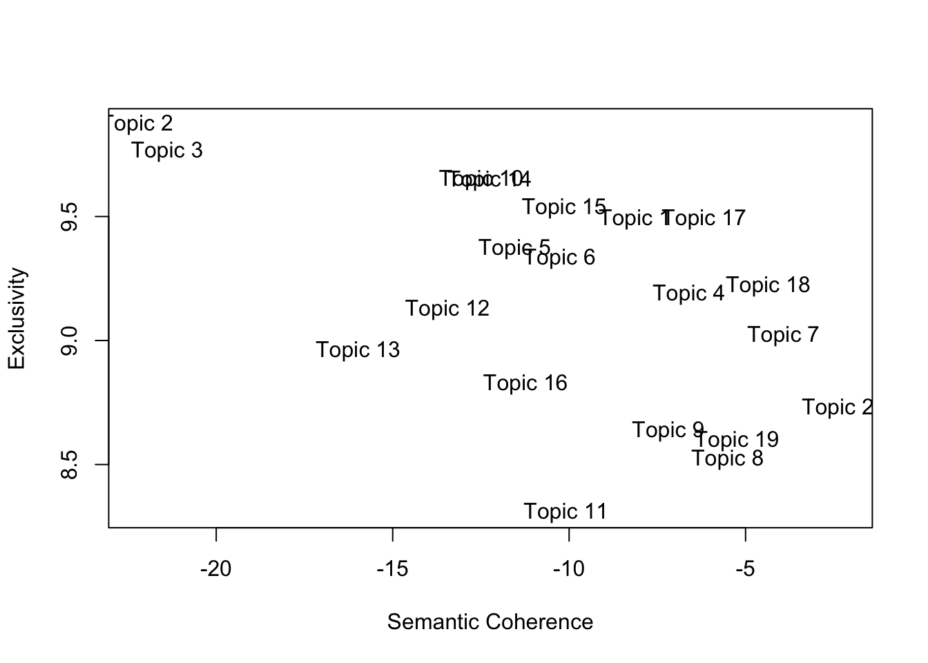

Maybe we have some theory about the difference in topic prevalence across parties. We can see the topic proportions in our topic model object:

head(stm_us_pres$theta)

##              [,1]         [,2]         [,3]         [,4]         [,5]
## [1,] 0.0001965139 8.910433e-05 8.224181e-05 1.366525e-04 0.0003038924
## [2,] 0.0004943115 6.694931e-05 9.823350e-01 1.233605e-04 0.0162390724
## [3,] 0.0002929573 4.935711e-05 9.988060e-01 1.794408e-05 0.0005358752
## [4,] 0.1143189826 9.475844e-04 8.765515e-01 2.637466e-04 0.0030686131
## [5,] 0.0117265212 2.101959e-04 6.658082e-03 1.163485e-03 0.9768804322
## [6,] 0.0254848264 3.421690e-04 4.654306e-03 1.751075e-03 0.9609666414
##              [,6]         [,7]         [,8]         [,9]        [,10]
## [1,] 2.109828e-04 1.271428e-04 9.985770e-01 1.726828e-04 1.037666e-04
## [2,] 1.673617e-04 1.837545e-04 2.369797e-04 9.412580e-05 5.907198e-05
## [3,] 6.424073e-05 5.105122e-05 6.933715e-05 6.752421e-05 4.572869e-05
## [4,] 7.946389e-04 8.965244e-04 7.116956e-04 1.080859e-03 1.365866e-03
## [5,] 5.210418e-04 4.736609e-04 8.391293e-04 8.456329e-04 6.818197e-04
## [6,] 7.226817e-04 6.610786e-04 1.740575e-03 1.314907e-03 2.361741e-03

Note that the prevalence terms \(\theta\) will add to 1 within a document. That is, the term tells us the proportion of (words associated with) topics for each document:

sum(stm_us_pres$theta[1,])

## [1] 1

sum(stm_us_pres$theta[2,])

## [1] 1

What about connecting this info to our dfm and seeing if there are differences in the proportion topic 5 (economy) is addressed by each side.

library(fixest)
library(sjPlot)

## #refugeeswelcome

us_pres_prev <- data.frame(topic5 = stm_us_pres$theta[,5], docvars(dfm_us_pres))
feols_topic5 <- feols(topic5 ~ party , data = us_pres_prev)
plot_model(feols_topic5, type = "pred", term = "party") +
  theme_minimal() +
  labs(caption = "Stat. Sig. at p<0.1", x="", y="Topic Prevalence")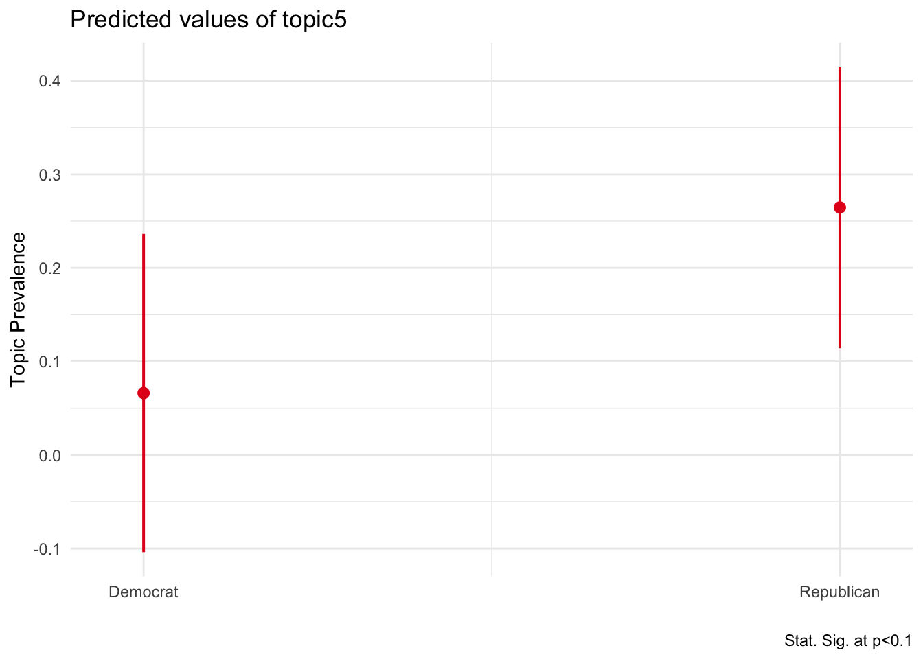

Seems that Republican presidents address more the economy in their speeches. Let’s plot the proportion of by president:

us_pres_prev %>%
  # Going to log the prev of topic 5 because is quite skewed but you should probably leave as is if you want to explore how topics are addressed. 
  ggplot(aes(x = log(topic5), y = reorder(President,topic5), color = party)) +
  geom_point(alpha = 0.8) +
  labs(x = "log(Theta)", y = "", color = "Party") +
  scale_color_manual(values = wes_palette("BottleRocket2")) +
  theme_minimal()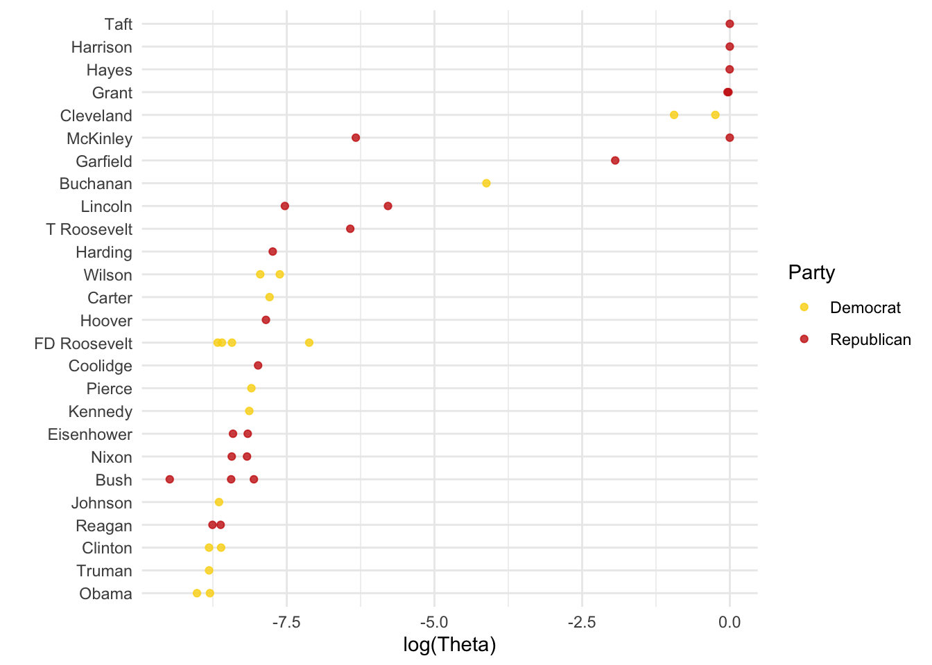

We can do something similar with the stm function directly. We just need to specify the functional form and add the document variables.

topics_us_pres <- estimateEffect(c(3,5) ~ party, stm_us_pres, docvars(dfm_us_pres)) # You can compare other topics by changing c(6,9). 
plot(topics_us_pres, "party", method = "difference",
     cov.value1 = "Democrat", 
     cov.value2 = "Republican",
     labeltype = "custom",
     xlim = c(-.75,.25),
     custom.labels = c('Topic 3: Slavery', 'Topic 5: Economy'),
     model = stm_us_pres)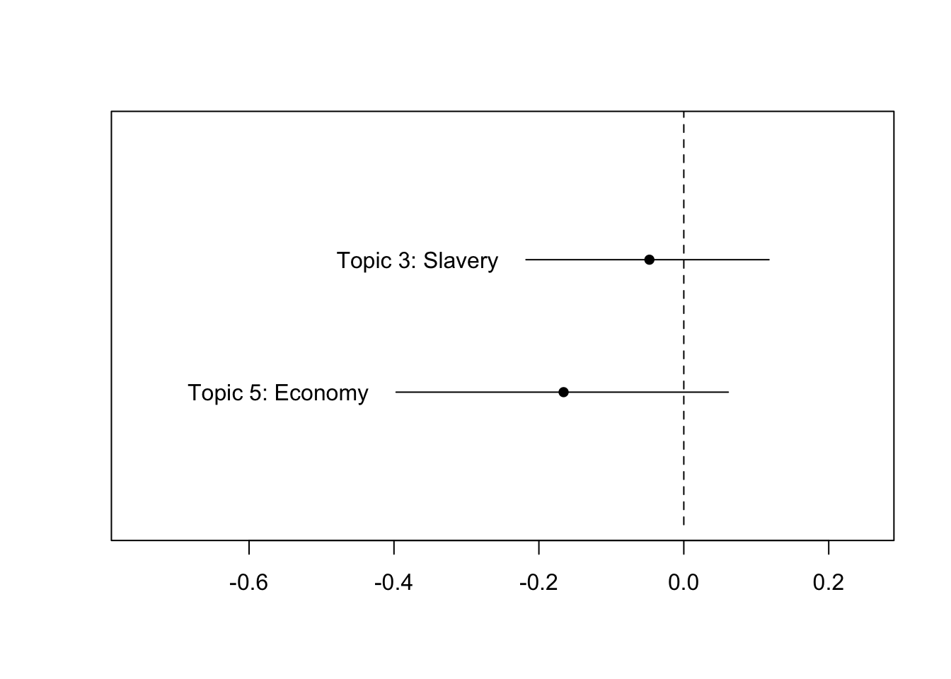

Same results, Republicans mention more Topic 5: Economy.

5.5 Homework 2:

We had a hard time scaling our text. Why looked at some possible problems. What are possible solutions if we want to position U.S. presidents in a ideological scale using text?
Use the data/candidate-tweets.csv data to run a STM. Decide what your covariates are going. Decide whether you will use all the data or a sample of the data. Decide if you are going to aggregate/divide in some way the text (i.e., decide your unit of analysis). Decide the number of topics you will look for (try more than one option). What can you tell me about the topics tweeted out by the 2015 U.S. primaries candidates?
Choose three topics. Can you place the candidates in an ideological scale within each topic (determine the \(theta\) threshold for when you can say that a tweet is mostly about a topic)? Does it make sense? Why or why not?

4 Week 4: Complexity and Similarity

6 Week 6: Word Embeddings