14 Lecture 5 Exercises

This tutorial was created by John Santos (with minor adaptations from me).

14.1 How to (nicely) display model results

If we want to display models in a more aesthetically-pleasing format than with the summary() command, we have a few options.

Let’s start by running some models.

library(wooldridge)
data("wage1")
wage_mod1<- lm(wage ~ educ + exper, data=wage1)
wage_mod1a<- lm(I(wage*100) ~ educ + exper, data=wage1)
wage_mod2 <- lm(wage ~ educ, data=wage1)

14.1.1 The boring, ugly way (Base R)

summary(wage_mod1)

## 
## Call:
## lm(formula = wage ~ educ + exper, data = wage1)
## 
## Residuals:
##     Min      1Q  Median      3Q     Max 
## -5.5532 -1.9801 -0.7071  1.2030 15.8370 
## 
## Coefficients:
##             Estimate Std. Error t value Pr(>|t|)    
## (Intercept) -3.39054    0.76657  -4.423 1.18e-05 ***
## educ         0.64427    0.05381  11.974  < 2e-16 ***
## exper        0.07010    0.01098   6.385 3.78e-10 ***
## ---
## Signif. codes:  0 '***' 0.001 '**' 0.01 '*' 0.05 '.' 0.1 ' ' 1
## 
## Residual standard error: 3.257 on 523 degrees of freedom
## Multiple R-squared:  0.2252, Adjusted R-squared:  0.2222 
## F-statistic: 75.99 on 2 and 523 DF,  p-value: < 2.2e-16

summary(wage_mod1a)

## 
## Call:
## lm(formula = I(wage * 100) ~ educ + exper, data = wage1)
## 
## Residuals:
##     Min      1Q  Median      3Q     Max 
## -555.32 -198.01  -70.71  120.30 1583.70 
## 
## Coefficients:
##             Estimate Std. Error t value Pr(>|t|)    
## (Intercept) -339.054     76.657  -4.423 1.18e-05 ***
## educ          64.427      5.381  11.974  < 2e-16 ***
## exper          7.010      1.098   6.385 3.78e-10 ***
## ---
## Signif. codes:  0 '***' 0.001 '**' 0.01 '*' 0.05 '.' 0.1 ' ' 1
## 
## Residual standard error: 325.7 on 523 degrees of freedom
## Multiple R-squared:  0.2252, Adjusted R-squared:  0.2222 
## F-statistic: 75.99 on 2 and 523 DF,  p-value: < 2.2e-16

summary(wage_mod2)

## 
## Call:
## lm(formula = wage ~ educ, data = wage1)
## 
## Residuals:
##     Min      1Q  Median      3Q     Max 
## -5.3396 -2.1501 -0.9674  1.1921 16.6085 
## 
## Coefficients:
##             Estimate Std. Error t value Pr(>|t|)    
## (Intercept) -0.90485    0.68497  -1.321    0.187    
## educ         0.54136    0.05325  10.167   <2e-16 ***
## ---
## Signif. codes:  0 '***' 0.001 '**' 0.01 '*' 0.05 '.' 0.1 ' ' 1
## 
## Residual standard error: 3.378 on 524 degrees of freedom
## Multiple R-squared:  0.1648, Adjusted R-squared:  0.1632 
## F-statistic: 103.4 on 1 and 524 DF,  p-value: < 2.2e-16

14.1.2 {stargazer}

The easiest is to use the {stargazer} package and its eponymously-named function. This package is easy enough, flexible enough, but, unfortunately, no longer maintained.

library(stargazer)

## 
## Please cite as:

##  Hlavac, Marek (2022). stargazer: Well-Formatted Regression and Summary Statistics Tables.

##  R package version 5.2.3. https://CRAN.R-project.org/package=stargazer

stargazer(wage_mod1, wage_mod1a, wage_mod2,
          title = "Modeling wage versus education and experience",
          type = "text")

## 
## Modeling wage versus education and experience
## ============================================================================================
##                                               Dependent variable:                           
##                     ------------------------------------------------------------------------
##                              wage                I(wage * 100)                wage          
##                               (1)                     (2)                     (3)           
## --------------------------------------------------------------------------------------------
## educ                       0.644***                64.427***                0.541***        
##                             (0.054)                 (5.381)                 (0.053)         
##                                                                                             
## exper                      0.070***                7.010***                                 
##                             (0.011)                 (1.098)                                 
##                                                                                             
## Constant                   -3.391***              -339.054***                -0.905         
##                             (0.767)                (76.657)                 (0.685)         
##                                                                                             
## --------------------------------------------------------------------------------------------
## Observations                  526                     526                     526           
## R2                           0.225                   0.225                   0.165          
## Adjusted R2                  0.222                   0.222                   0.163          
## Residual Std. Error    3.257 (df = 523)       325.704 (df = 523)        3.378 (df = 524)    
## F Statistic         75.990*** (df = 2; 523) 75.990*** (df = 2; 523) 103.363*** (df = 1; 524)
## ============================================================================================
## Note:                                                            *p<0.1; **p<0.05; ***p<0.01

For {stargazer}, you want to set the type= option to “text” while you work in RStudio, but change it to “html” or “latex” when you output your final document (respectively, as an HTML file or .tex file).

14.1.3 {modelsummary}

We can also use the package modelsummary and its function msummary(). This package is a little more involved, but produces a more flexible output, works with a wider variety of models, and is actively maintained.

library(modelsummary)

## `modelsummary` 2.0.0 now uses `tinytable` as its default table-drawing backend. Learn more at:
##   https://vincentarelbundock.github.io/tinytable/
## 
## Revert to `kableExtra` for one session:
## 
##   options(modelsummary_factory_default = 'kableExtra')
##   options(modelsummary_factory_latex = 'kableExtra')
##   options(modelsummary_factory_html = 'kableExtra')
## 
## Silence this message forever:
## 
##   config_modelsummary(startup_message = FALSE)

## 
## Attaching package: 'modelsummary'

## The following object is masked from 'package:psych':
## 
##     SD

msummary(models = dvnames(list(wage_mod1, wage_mod1a, wage_mod2)),
         statistic = c("std.error", "p.value"),
         stars = TRUE,
         title = "Modeling wage versus education and experience",
         notes = "Cell entries are parameter estimates, standard errors, and p values")

Modeling wage versus education and experience

	wage	I(wage * 100)	wage
+ p
Cell entries are parameter estimates, standard errors, and p values
(Intercept)	-3.391***	-339.054***	-0.905
	(0.767)	(76.657)	(0.685)
	(	(	(0.187)
educ	0.644***	64.427***	0.541***
	(0.054)	(5.381)	(0.053)
	(	(	(
exper	0.070***	7.010***
	(0.011)	(1.098)
	(	(
Num.Obs.	526	526	526
R2	0.225	0.225	0.165
R2 Adj.	0.222	0.222	0.163
AIC	2739.9	7584.6	2777.4
BIC	2757.0	7601.6	2790.2
Log.Lik.	-1365.969	-3788.288	-1385.712
F	75.990	75.990	103.363
RMSE	3.25	324.77	3.37

---

14.2 Functional form

14.2.1 Feelings towards the LPC (quadratics)

Quadratics on the right-hand-side (RHS) of a regression equation are useful for capturing non-linear relationships, especially when that relationship is non-monotonic.

When a function is non-monotonic, it means that it switches direction (either positive to negative or negative to positive).

We’ll demonstrate this by modelling feelings towards the Liberal Party of Canada and market liberalism.

load("Sample_data/ces.rda")

summary(ces$marketlib)

##    Min. 1st Qu.  Median    Mean 3rd Qu.    Max.    NA's 
##    0.00    6.00    9.00    8.59   11.00   16.00   32684

summary(ces$feel_lib)

##    Min. 1st Qu.  Median    Mean 3rd Qu.    Max.    NA's 
##    0.00   16.00   54.00   48.34   77.00  100.00    2640

ggplot(ces) +
  aes(x = feel_lib, y = marketlib) +
  geom_point(position = "jitter") +
  geom_smooth(method = "lm") +
  geom_smooth(method = "lm", 
              formula = "y ~ x + I(x^2)", 
              color = "red")

## `geom_smooth()` using formula = 'y ~ x'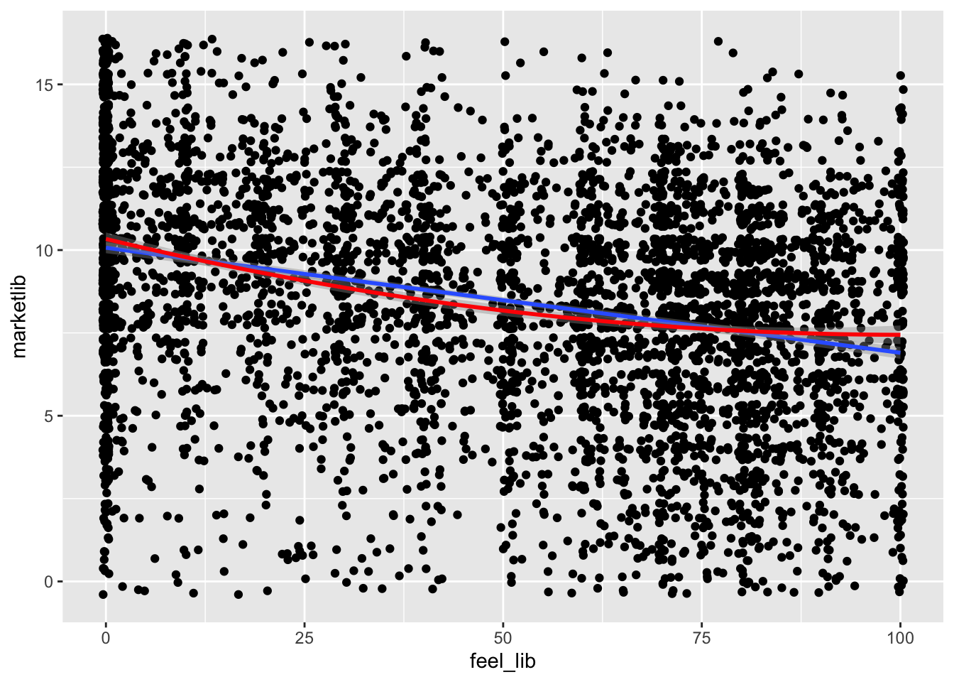

feel1 <- lm(feel_lib ~ marketlib, data = ces)
feel2 <- lm(feel_lib ~ marketlib + I(marketlib^2), data = ces)

stargazer(feel1, feel2,
          type = "text")

## 
## =======================================================================
##                                     Dependent variable:                
##                     ---------------------------------------------------
##                                          feel_lib                      
##                                (1)                       (2)           
## -----------------------------------------------------------------------
## marketlib                   -2.802***                   0.654          
##                              (0.130)                   (0.481)         
##                                                                        
## I(marketlib2)                                         -0.216***        
##                                                        (0.029)         
##                                                                        
## Constant                    71.472***                 60.439***        
##                              (1.203)                   (1.904)         
##                                                                        
## -----------------------------------------------------------------------
## Observations                  4,781                     4,781          
## R2                            0.089                     0.099          
## Adjusted R2                   0.089                     0.099          
## Residual Std. Error    31.808 (df = 4779)        31.628 (df = 4778)    
## F Statistic         466.091*** (df = 1; 4779) 263.454*** (df = 2; 4778)
## =======================================================================
## Note:                                       *p<0.1; **p<0.05; ***p<0.01

The effect of X on Y, or of marketlib on feel_lib requires both $\widehat{{\beta }_1}$ and $\widehat{{\beta }_2}$, as can be seen below.

$$\begin{array}{rl}\widehat{feellib}& =60.439+0.654marketlib-0.216marketli{b}^2\\ \mathrm{\Delta }\widehat{feellib}& =0.654marketlib-0.216marketli{b}^2\end{array}$$

The above has a convenient approximation of , which is applied as follows:

$$\begin{array}{rl}\mathrm{\Delta }\hat{y}& =\widehat{{\beta }_1}x+\widehat{{\beta }_2}{x}^2\\ \mathrm{\Delta }\hat{y}& \approx [\widehat{{\beta }_1}+(2\times \widehat{{\beta }_2}x)]\mathrm{\Delta }x\\ \mathrm{\Delta }\widehat{feellib}& \approx [0.654-(2\times 0.216marketlib)]\mathrm{\Delta }marketlib\\ \mathrm{\Delta }\widehat{feellib}& \approx [0.654-0.432marketlib]\mathrm{\Delta }marketlib\\ \mathrm{\Delta }marketlib& =1& & \text{(because we're looking at a one-unit change in marketlib)}\\ \mathrm{\Delta }\widehat{feellib}& \approx [0.654-0.432marketlib]\end{array}$$

14.2.1.1 Calculating the turning point of a quadratic

The point (at least theoretically) at which a quadratic function changes direction is called the turning point, or the inflection point, or a functional minimum/maximum. It is often represented as $x\star$.

Another way to think about this is the point at which the rate of change of Y across values of X equals 0, or more formally $\mathrm{\Delta }\hat{y}=0$.

For quadratic equations of $\hat{y}={\hat{\beta }}_0+{\hat{\beta }}_{1}x+{\hat{\beta }}_2{x}^2$ this point can be calculated with the formula $x\star =-{\hat{\beta }}_1/2{\hat{\beta }}_2$.

For the example above, this point is $$\begin{array}{rl}x\star & =-{\hat{\beta }}_1/2{\hat{\beta }}_2\\ x\star & =-0.654/(2\times 0.216)\\ x\star & =-0.654/0.432\\ x\star & =-1.513889\end{array}$$

So, the turning point at which a one-unit change in marketlib causes feelings towards the LPC to change direction is -1.5. This is outside of the actual range of the marketlib variable, so it is of no relevance to us (hence why the turning point is sometimes only theoretical).

You’ll encounter this later in the course, so don’t worry about this too much at this point.

---

14.2.2 Occupational prestige (logarithms)

Logarithms are useful on both the right- (predictor) and left-hand-side (outcome) of regression equations.

The log of $X$ is useful when that predictor has large effects on $Y$ at low levels of $X$ but smaller effects at higher levels of $X$.

It can also be useful in the converse situation.

library(tidyverse)
library(ggplot2)
library(carData)
data(Prestige)

summary(Prestige)

##    education          income          women           prestige         census       type   
##  Min.   : 6.380   Min.   :  611   Min.   : 0.000   Min.   :14.80   Min.   :1113   bc  :44  
##  1st Qu.: 8.445   1st Qu.: 4106   1st Qu.: 3.592   1st Qu.:35.23   1st Qu.:3120   prof:31  
##  Median :10.540   Median : 5930   Median :13.600   Median :43.60   Median :5135   wc  :23  
##  Mean   :10.738   Mean   : 6798   Mean   :28.979   Mean   :46.83   Mean   :5402   NA's: 4  
##  3rd Qu.:12.648   3rd Qu.: 8187   3rd Qu.:52.203   3rd Qu.:59.27   3rd Qu.:8312            
##  Max.   :15.970   Max.   :25879   Max.   :97.510   Max.   :87.20   Max.   :9517

ggplot(Prestige) +
  aes(x = income, y = prestige) +
  geom_point(position = "jitter") +
  geom_smooth(method = "lm") +
  labs(title = "prestige ~ income")

## `geom_smooth()` using formula = 'y ~ x'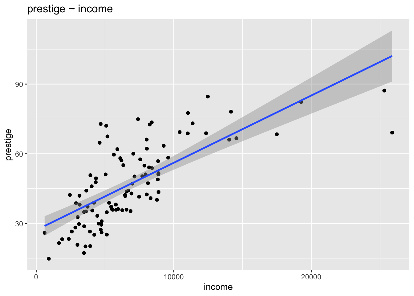

prest1 <- lm(prestige ~ income, data = Prestige)

summary(prest1)

## 
## Call:
## lm(formula = prestige ~ income, data = Prestige)
## 
## Residuals:
##     Min      1Q  Median      3Q     Max 
## -33.007  -8.378  -2.378   8.432  32.084 
## 
## Coefficients:
##              Estimate Std. Error t value Pr(>|t|)    
## (Intercept) 2.714e+01  2.268e+00   11.97   <2e-16 ***
## income      2.897e-03  2.833e-04   10.22   <2e-16 ***
## ---
## Signif. codes:  0 '***' 0.001 '**' 0.01 '*' 0.05 '.' 0.1 ' ' 1
## 
## Residual standard error: 12.09 on 100 degrees of freedom
## Multiple R-squared:  0.5111, Adjusted R-squared:  0.5062 
## F-statistic: 104.5 on 1 and 100 DF,  p-value: < 2.2e-16

$$\widehat{prestige}=2.714+0.002897income$$

For every increase in income of $1, prestige increases by about 0.002897 points on a scale from 14 to 87 points.

Alternatively, for every increase in $1000, prestige increases by about 2.9 points (0.002897 * 1000 = 2.897).

BUT…, is the relationship actually linear?

ggplot(Prestige) +
  aes(x = income, y = prestige) +
  geom_point(position = "jitter") +
  geom_smooth(method = "lm") +
  geom_smooth(method = "lm", formula = "y ~ log(x)", color = "red") +
  labs(title = "prestige ~ income")

## `geom_smooth()` using formula = 'y ~ x'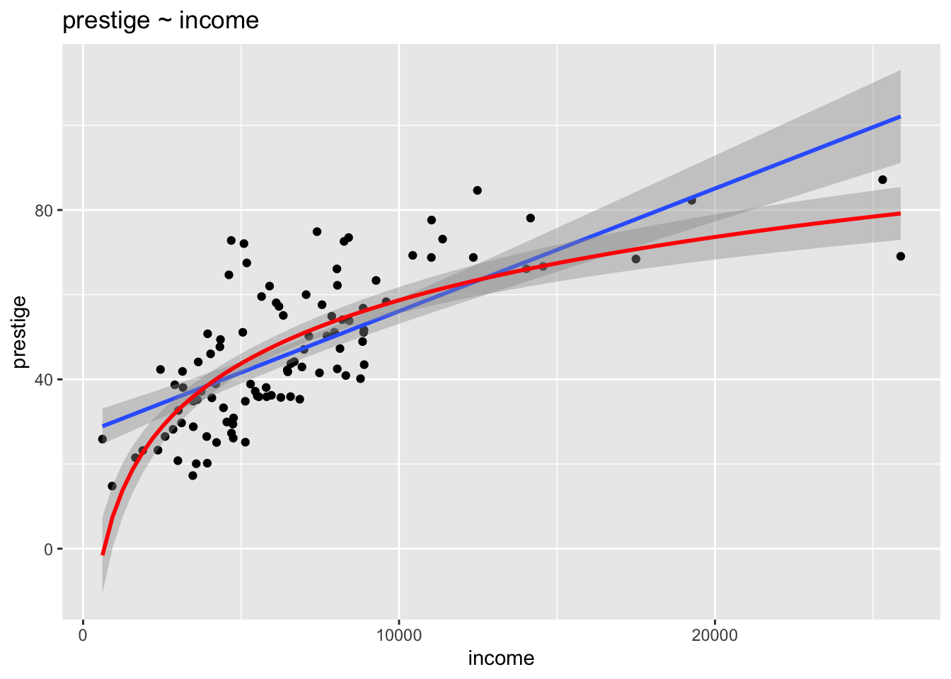

It looks like a logarithmic function might work better, so let’s try that.

To make the coefficients easier to interpret, we’ll make a new variable that is a transformation of income, but measured in thousands.

Prestige$income1000 <- Prestige$income / 1000
prest1 <- lm(prestige ~ income1000, data = Prestige)
prest2 <- lm(prestige ~ log(income1000), data = Prestige)
prest3 <- lm(log(prestige) ~ income1000, data = Prestige)
prest4 <- lm(log(prestige) ~ log(income1000), data = Prestige)

library(stargazer)
stargazer(prest1, prest2, prest3, prest4,
          type = "text")

## 
## =========================================================================
##                                           Dependent variable:            
##                                ------------------------------------------
##                                      prestige           log(prestige)    
##                                   (1)        (2)        (3)       (4)    
## -------------------------------------------------------------------------
## income1000                      2.897***             0.062***            
##                                 (0.283)               (0.007)            
##                                                                          
## log(income1000)                           21.556***             0.499*** 
##                                            (1.953)              (0.044)  
##                                                                          
## Constant                       27.141***   9.050**   3.353***   2.901*** 
##                                 (2.268)    (3.611)    (0.055)   (0.081)  
##                                                                          
## -------------------------------------------------------------------------
## Observations                      102        102        102       102    
## R2                               0.511      0.549      0.452     0.566   
## Adjusted R2                      0.506      0.545      0.447     0.562   
## Residual Std. Error (df = 100)   12.090     11.609     0.291     0.259   
## F Statistic (df = 1; 100)      104.537*** 121.810*** 82.642*** 130.520***
## =========================================================================
## Note:                                         *p<0.1; **p<0.05; ***p<0.01

$$\begin{array}{rlrl}\widehat{prestige}& =27.141+2.897income& & \text{(eq 1: level-level)}\\ \widehat{prestige}& =9.050+21.556log(income)& & \text{(eq 2: level-log)}\\ \widehat{log(prestige)}& =3.353+0.062income& & \text{(eq 3: log-level)}\\ \widehat{log(prestige)}& =2.901+0.499log(income)& & \text{(eq 4: log-log)}\end{array}$$

Remembering our rules for interpreting models, which are…

1. level-level A unit increase in X results in a b unit increase in Y
2. level-log A percent increase in X results in a (b/100)*unit increase in Y
3. log-level A unit increase in X results in a 100*b% increase in Y
4. log-log A percent increase in X results in a b% increase in Y

Therefore, the interpretation of each equation is as follows:

1. For every increase in income of $1 (thousand), prestige increases by about 2.897 points.
2. For every 1% increase in income (in thousands), prestige increases by .21556 points (i.e. ${\hat{\beta }}_1/100=21.556/100==0.21556$).
3. For every increase in income of $1 (thousand), prestige increases 6.2% (i.e. $100\ast {\hat{\beta }}_1=0.062/100==6.2\mathrm{\%}$).
4. For every 1% increase in income (in thousands), prestige increases by 0.499%.

p1 <- ggplot(Prestige) +
  aes(x = income, y = prestige) +
  geom_point(position = "jitter") +
  geom_smooth(method = "lm") +
  labs(title = "prestige ~ income")

p2 <- ggplot(Prestige) +
  aes(x = log(income), y = prestige) +
  geom_point(position = "jitter") +
  geom_smooth(method = "lm") +
  labs(title = "prestige ~ log(income)")

p3 <- ggplot(Prestige) +
  aes(x = income, y = log(prestige)) +
  geom_point(position = "jitter") +
  geom_smooth(method = "lm") +
  labs(title = "log(prestige) ~ income")

p4 <- ggplot(Prestige) +
  aes(x = log(income), y = log(prestige)) +
  geom_point(position = "jitter") +
  geom_smooth(method = "lm") +
  labs(title = "log(prestige) ~ log(income)")

library(ggpubr)

## 
## Attaching package: 'ggpubr'

## The following objects are masked from 'package:tidylog':
## 
##     group_by, mutate

ggarrange(p1, p2, p3, p4)

## `geom_smooth()` using formula = 'y ~ x'

## `geom_smooth()` using formula = 'y ~ x'
## `geom_smooth()` using formula = 'y ~ x'
## `geom_smooth()` using formula = 'y ~ x'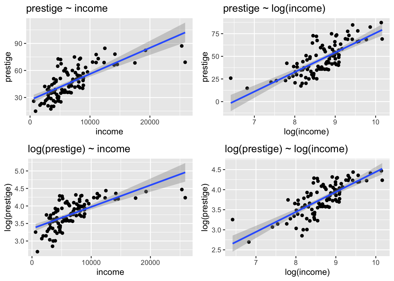

---

14.2.3 Automobile performance (logarithms)

This is another exercise using the the mtcars dataset from the carData package. We’ll model quarter-mile time (qsec) as a function of horsepower (hp).

library(tidyverse)
library(ggplot2)
data(mtcars)

summary(mtcars)

##       mpg             cyl             disp             hp             drat             wt             qsec      
##  Min.   :10.40   Min.   :4.000   Min.   : 71.1   Min.   : 52.0   Min.   :2.760   Min.   :1.513   Min.   :14.50  
##  1st Qu.:15.43   1st Qu.:4.000   1st Qu.:120.8   1st Qu.: 96.5   1st Qu.:3.080   1st Qu.:2.581   1st Qu.:16.89  
##  Median :19.20   Median :6.000   Median :196.3   Median :123.0   Median :3.695   Median :3.325   Median :17.71  
##  Mean   :20.09   Mean   :6.188   Mean   :230.7   Mean   :146.7   Mean   :3.597   Mean   :3.217   Mean   :17.85  
##  3rd Qu.:22.80   3rd Qu.:8.000   3rd Qu.:326.0   3rd Qu.:180.0   3rd Qu.:3.920   3rd Qu.:3.610   3rd Qu.:18.90  
##  Max.   :33.90   Max.   :8.000   Max.   :472.0   Max.   :335.0   Max.   :4.930   Max.   :5.424   Max.   :22.90  
##        vs               am              gear            carb      
##  Min.   :0.0000   Min.   :0.0000   Min.   :3.000   Min.   :1.000  
##  1st Qu.:0.0000   1st Qu.:0.0000   1st Qu.:3.000   1st Qu.:2.000  
##  Median :0.0000   Median :0.0000   Median :4.000   Median :2.000  
##  Mean   :0.4375   Mean   :0.4062   Mean   :3.688   Mean   :2.812  
##  3rd Qu.:1.0000   3rd Qu.:1.0000   3rd Qu.:4.000   3rd Qu.:4.000  
##  Max.   :1.0000   Max.   :1.0000   Max.   :5.000   Max.   :8.000

hpqsec1 <- lm(qsec ~ hp, data = mtcars)
hpqsec2 <- lm(qsec ~ log(hp), data = mtcars)
hpqsec3 <- lm(log(qsec) ~ hp, data = mtcars)
hpqsec4 <- lm(log(qsec) ~ log(hp), data = mtcars)

library(stargazer)
stargazer(hpqsec1, hpqsec2, hpqsec3, hpqsec4,
          type = "text")

## 
## =====================================================================
##                                         Dependent variable:          
##                               ---------------------------------------
##                                      qsec              log(qsec)     
##                                  (1)       (2)       (3)       (4)   
## ---------------------------------------------------------------------
## hp                            -0.018***           -0.001***          
##                                (0.003)            (0.0002)           
##                                                                      
## log(hp)                                 -2.576***           -0.146***
##                                          (0.500)             (0.027) 
##                                                                      
## Constant                      20.556*** 30.422*** 3.032***  3.591*** 
##                                (0.542)   (2.453)   (0.029)   (0.134) 
##                                                                      
## ---------------------------------------------------------------------
## Observations                     32        32        32        32    
## R2                              0.502     0.469     0.530     0.488  
## Adjusted R2                     0.485     0.451     0.515     0.471  
## Residual Std. Error (df = 30)   1.282     1.323     0.069     0.072  
## F Statistic (df = 1; 30)      30.190*** 26.514*** 33.882*** 28.575***
## =====================================================================
## Note:                                     *p<0.1; **p<0.05; ***p<0.01

ggplot(mtcars) +
  aes(x = hp, y = qsec) +
  geom_point(position = "jitter") +
  geom_smooth(method = "lm") +
  geom_smooth(method = "lm", formula = y ~ log(x), color = "red") +
  labs(title = "qsec ~ hp")

## `geom_smooth()` using formula = 'y ~ x'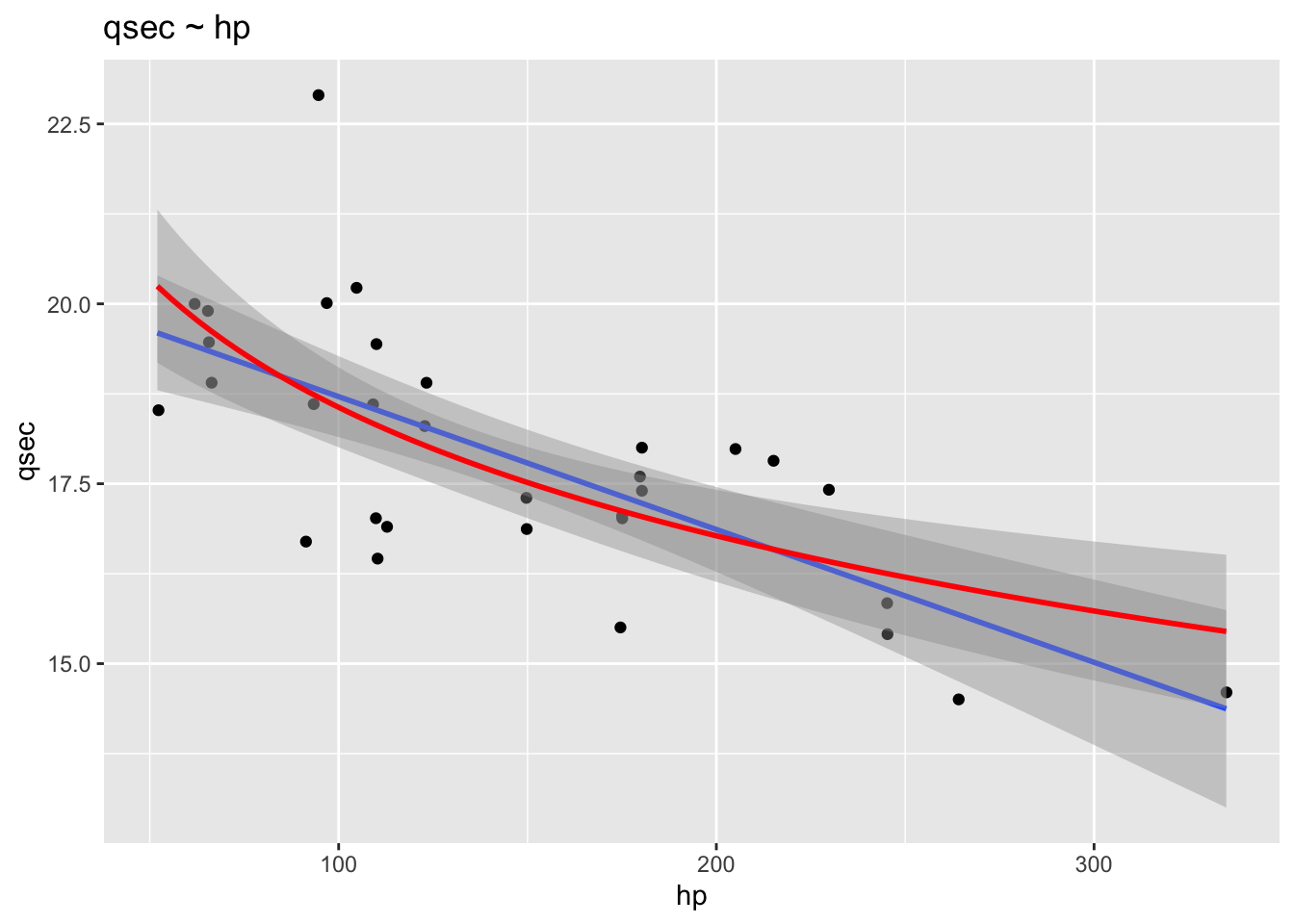

ggplot(mtcars) +
  aes(x = hp, y = log(qsec)) +
  geom_point(position = "jitter") +
  geom_smooth(method = "lm", formula = y ~ x) +
  labs(title = "log(qsec) ~ hp")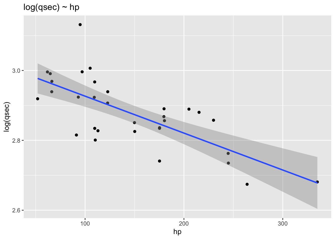

ggplot(mtcars) +
  aes(x = log(hp), y = log(qsec)) +
  geom_point(position = "jitter") +
  geom_smooth(method = "lm", formula = y ~ x) +
  labs(title = "log(qsec) ~ log(hp)")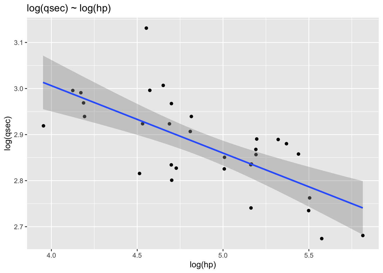

---

14.3 Practice exercises

From lecture:

Using the ‘fertil2’ dataset from ‘wooldridge’ on women living in the Republic of Botswana in 1988…

1. Estimate the regression equation of the number of children on education, age of the mother, and electricity.
2. Interpret ${\hat{\beta }}_0$, ${\hat{\beta }}_{education}$, ${\hat{\beta }}_{age}$, and ${\hat{\beta }}_{electric}$.
3. Verify that sample covariance between predicted values and residuals = 0.
4. Verify that sample covariance between education and residuals = 0.
5. Re-estimate the regression equation of the number of children on education, age of the mother, and electricity but also include the square of the age of the mother. How do you now interpret the effect of age on the number of children?

Using the ‘wage1’ datadest from ‘woolridge’ on US workers in 1976…

6. Estimate the regression equation of the hourly wage (wage) in dollars on education (educ) and experience (exper).
7. How do the coefficients change when the units of wages are in cents instead of dollars?
8. Compare the estimated coefficient for education to the one obtained by regressing only the hourly wage on education. Interpret.

Additional exercises for tutorial:

There’s an old saying (often attributed to Winston Churchill) that goes, “If you are not a liberal when you are young, you have no heart. If you are not a conservative when you are old, you have no brain.” And, yet there have been activist left-wing groups comprised of seniors, like the Raging Grannies.

Using our sample CES dataset, explore the relationship between Canadians’ support for free market principles ($marketlib$) and age ($age$)? Is there is a relationship? If so, is it linear? We’re going to run two regression models. Model 1 will regress $marketlib$ on $age$, while controlling for $gender$. Model 2 will be the same as Model 1, except it will also include the quadratic term for $age$ (i.e. $ag{e}^2$).

14.4 STOP!!

Before you continue, try solving the exercises on your own. It’s the only way you will learn. Then, come back to this page and see how well you did.

14.5 Continue

14.6 Lecture exercises

14.6.1 Q1. Estimate the regression equation of the number of children on education, age of the mother, and electricity.

Before I begin, I’m going to make a data frame that only contains the variables I need and then listiwise delete all NAs. This will make it easier to run the diagnostic tests.

library(wooldridge)
library(tidyverse)
data("fertil2")
dat <- fertil2 %>%
  select(c(children, educ, age, electric)) %>%
  na.omit()

## select: dropped 23 variables (mnthborn, yearborn, radio, tv, bicycle, …)

Our population model is:

$$children={\beta }_0+{\beta }_{1}educ+{\beta }_{2}age+{\beta }_{3}electric+u$$

library(wooldridge)
fertil2 <- get(data('fertil2'))
library(dplyr)

fmod1 <- lm(children ~ educ + age + electric, data = dat)

summary(fmod1)

## 
## Call:
## lm(formula = children ~ educ + age + electric, data = dat)
## 
## Residuals:
##     Min      1Q  Median      3Q     Max 
## -6.6019 -0.6814 -0.0619  0.7476  7.1061 
## 
## Coefficients:
##              Estimate Std. Error t value Pr(>|t|)    
## (Intercept) -2.071091   0.094741 -21.861  < 2e-16 ***
## educ        -0.078751   0.006319 -12.462  < 2e-16 ***
## age          0.176999   0.002729  64.855  < 2e-16 ***
## electric    -0.361758   0.068032  -5.317  1.1e-07 ***
## ---
## Signif. codes:  0 '***' 0.001 '**' 0.01 '*' 0.05 '.' 0.1 ' ' 1
## 
## Residual standard error: 1.471 on 4354 degrees of freedom
## Multiple R-squared:  0.5621, Adjusted R-squared:  0.5618 
## F-statistic:  1863 on 3 and 4354 DF,  p-value: < 2.2e-16

Our model returns a regression equation of:

$$\widehat{children}=-2.071-0.079educ+0.177age-0.362electric$$

$$\begin{gathered} n=4,358 \\ {R}^2=0.562 \end{gathered}$$

14.6.2 Q2. Interpret ${\hat{\beta }}_0$, ${\hat{\beta }}_{education}$, ${\hat{\beta }}_{age}$, and ${\hat{\beta }}_{electric}$

$\widehat{{\beta }_0}$: This is the intercept, or the average predicted number of children when all three predictors are set to zero. It is -2.07 and is not theoretically meaningful (as you cannot have negative children).

${\hat{\beta }}_{education}$: For every additional year of education a woman has, we would predict her to have, on average, -0.08 fewer children, holding all other things constant.

${\hat{\beta }}_{age}$: For every additional year of age, we would predict a woman to have, on average, 0.18 more children, ceteris paribus.

${\hat{\beta }}_{electric}$: Women with electricity have, on average, 0.36 fewer children than women without electricity, ceteris paribus.

14.6.3 Q3. Verify that sample covariance between predicted values and residuals = 0.

There are two ways to do this. Mathematically, we can use the cov() command with the fitted values and residuals as inputs into the function.

cov(fmod1$fitted.values, fmod1$residuals)

## [1] -3.381377e-16

cov(fitted(fmod1), resid(fmod1))

## [1] -3.381377e-16

While the covariance is not exactly 0, the number is so small, it is basically zero.

Note, finding the correlation between fitted values and residuals gets us to the same answer because a correlation coefficient is simply a mathematical transformation of the covariance that bounds the result to [-1,1].

cor.test(fmod1$fitted.values, fmod1$residuals)

## 
##  Pearson's product-moment correlation
## 
## data:  fmod1$fitted.values and fmod1$residuals
## t = -9.1115e-15, df = 4356, p-value = 1
## alternative hypothesis: true correlation is not equal to 0
## 95 percent confidence interval:
##  -0.0296911  0.0296911
## sample estimates:
##           cor 
## -1.380524e-16

You might remember from earlier stats classes that

$$correlation=\frac{covariance(x,y)}{{\sigma }_x{\sigma }_y}$$

So, the result of calculating the above equation manually should equal that of using the cor() command

cov(fmod1$fitted.values, fmod1$residuals) / (sd(fmod1$fitted.values) * sd(fmod1$residuals))

## [1] -1.380524e-16

We can also confirm that there is no relationship between the fitted values and residuals by plotting them.

(This is called a “residual versus fitted/predicted plot” and is a very useful tool in diagnosing models for potential problems like non-linearity, heteroskedasticity, and outliers. )

library(ggplot2)
ggplot() + 
  aes(x = fmod1$fitted.values, y = fmod1$residuals) +
  geom_point(position = "jitter") + 
  labs(x = "Predicted number of children", 
       y = "Residual",
       title = "Predicted versus residual plot") + 
  geom_smooth(method = "lm", se = FALSE)

## `geom_smooth()` using formula = 'y ~ x'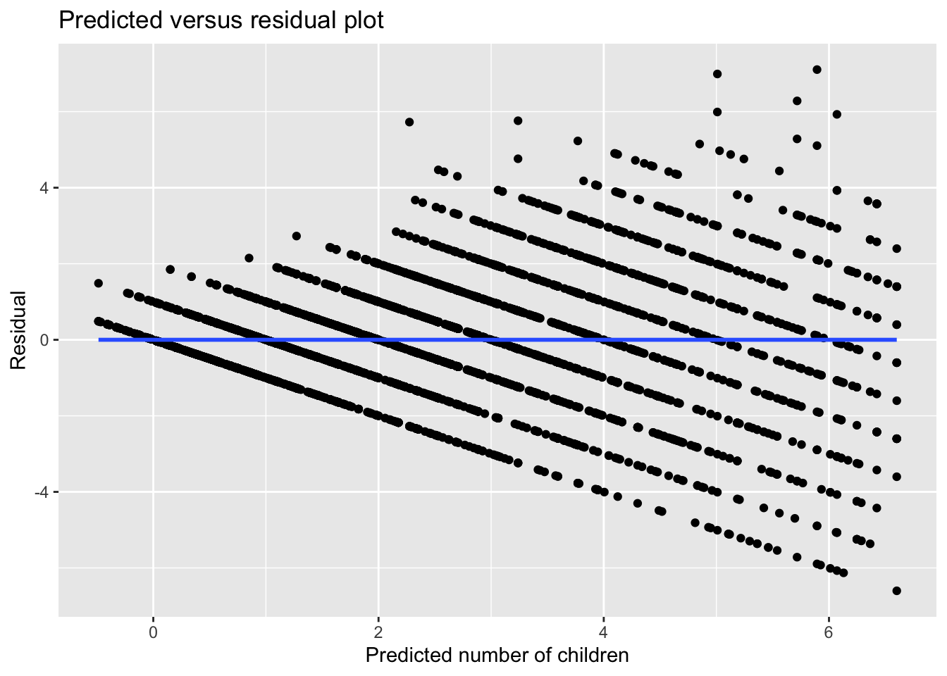

14.6.4 Q4. Verify that sample covariance between education and residuals = 0.

We’ll do the same here as we did with the fitted versus residuals. First, we’ll use R to calculate the covariance.

cov(dat$educ, resid(fmod1))

## [1] 1.216786e-15

As with before, this number is not exactly zero, but it is basically zero.

We can confirm this with visual inspection.

ggplot() + 
  aes(x = dat$educ, y = fmod1$residuals) +
  geom_point(position = "jitter") + 
  labs(x = "Education", 
       y = "Residual",
       title = "Education versus residual plot") + 
  geom_smooth(method = "lm", se = FALSE)

## `geom_smooth()` using formula = 'y ~ x'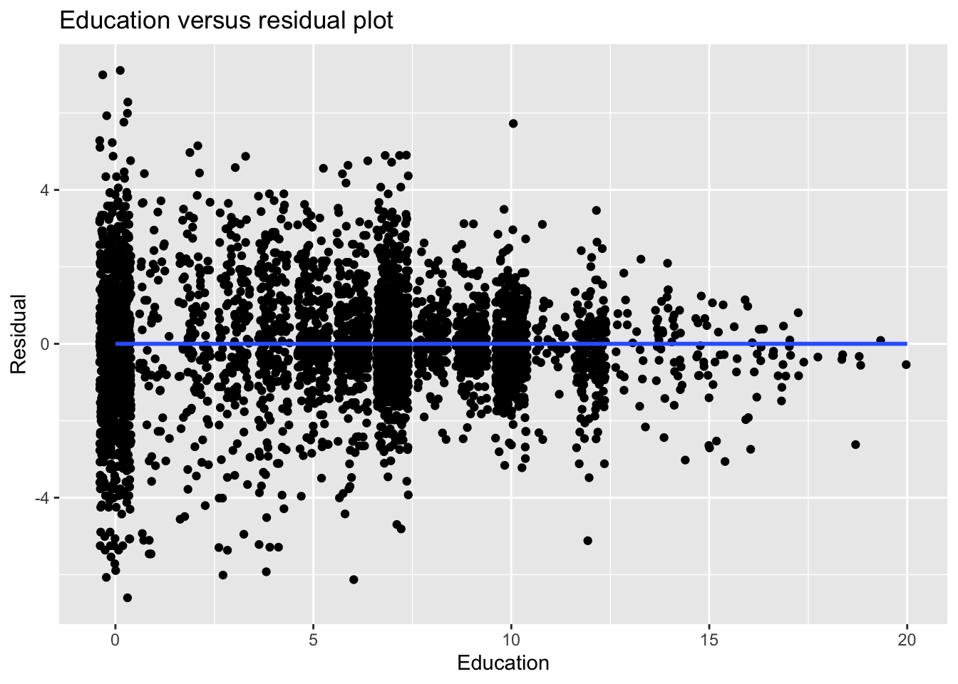

14.6.5 Q5. Re-estimate the regression equation of the number of children on education, age of the mother, and electricity but also include the square of the age of the mother. How do you now interpret the effect of age on the number of children?

Our population model is:

$$children={\beta }_0+{\beta }_{1}educ+{\beta }_{2}age+{\beta }_{3}ag{e}^2+{\beta }_{4}electric+u$$

To include $ag{e}^2$ in the model, we can enclose it in parentheses and preface it with a capital “I” (i.e. I(age^2)). This tells the lm() command to calculate whatever is inside I().

fmod2 <- lm(children ~ educ + age + I(age^2) + electric, data = dat)
summary(fmod2)

## 
## Call:
## lm(formula = children ~ educ + age + I(age^2) + electric, data = dat)
## 
## Residuals:
##     Min      1Q  Median      3Q     Max 
## -5.8576 -0.7153 -0.0005  0.7186  7.4868 
## 
## Coefficients:
##               Estimate Std. Error t value Pr(>|t|)    
## (Intercept) -4.2475679  0.2406003 -17.654  < 2e-16 ***
## educ        -0.0788944  0.0062513 -12.620  < 2e-16 ***
## age          0.3370397  0.0165166  20.406  < 2e-16 ***
## I(age^2)    -0.0026696  0.0002718  -9.822  < 2e-16 ***
## electric    -0.3777901  0.0673176  -5.612 2.12e-08 ***
## ---
## Signif. codes:  0 '***' 0.001 '**' 0.01 '*' 0.05 '.' 0.1 ' ' 1
## 
## Residual standard error: 1.455 on 4353 degrees of freedom
## Multiple R-squared:  0.5716, Adjusted R-squared:  0.5712 
## F-statistic:  1452 on 4 and 4353 DF,  p-value: < 2.2e-16

Our model returns a regression equation of:

$$\widehat{children}=-4.248-0.079educ+0.337age-0.0027ag{e}^2-0.362electric$$ $$\begin{gathered} n=4,358 \\ {R}^2=0.572 \end{gathered}$$

Adding the quadratic (i.e. squared) term for age to the model returns a positive coefficient for $age$ and a negative coefficient for $ag{e}^2$. This means that there is a positive relationship between age and the predicted number of children up until a point, and then the relationship becomes negative.

You can check this result by using a graphing calculator app like Desmos (https://www.desmos.com/calculator) and entering a function that only includes the terms for $age$ and $ag{e}^2$ (i.e. you would enter $y=0.337x-0.0027x^2$ into the app).

---

Using the ‘wage1’ datadest from ‘woolridge’ on US workers in 1976…

14.6.6 Q6. Estimate the regression equation of the hourly wage ($wage$) in dollars on education ($educ$) and experience ($exper$).

Our population model is:

$$wage={\beta }_0+{\beta }_{1}educ+{\beta }_{2}exper+u$$

library(wooldridge)
data("wage1")
wage_mod1<- lm(wage ~ educ + exper, data=wage1)
summary(wage_mod1)

## 
## Call:
## lm(formula = wage ~ educ + exper, data = wage1)
## 
## Residuals:
##     Min      1Q  Median      3Q     Max 
## -5.5532 -1.9801 -0.7071  1.2030 15.8370 
## 
## Coefficients:
##             Estimate Std. Error t value Pr(>|t|)    
## (Intercept) -3.39054    0.76657  -4.423 1.18e-05 ***
## educ         0.64427    0.05381  11.974  < 2e-16 ***
## exper        0.07010    0.01098   6.385 3.78e-10 ***
## ---
## Signif. codes:  0 '***' 0.001 '**' 0.01 '*' 0.05 '.' 0.1 ' ' 1
## 
## Residual standard error: 3.257 on 523 degrees of freedom
## Multiple R-squared:  0.2252, Adjusted R-squared:  0.2222 
## F-statistic: 75.99 on 2 and 523 DF,  p-value: < 2.2e-16

Our model returns a regression equation of:

$$\widehat{wage}=-3.391-0.644educ+0.070exper$$ $$\begin{gathered} n=526 \\ {R}^2=0.225 \end{gathered}$$

The terms are:

• ${\hat{\beta }}_0$ : This is the intercept, or the predicted wage when all education and experience are both zero. three predictors are set to zero. It is -3.39 and is not theoretically meaningful (as one does not typically pay to work).
• ${\hat{\beta }}_{educ}$ : For every additional year of education a worker has, we would predict them to make, on average, an additional $0.64 per hour, ceteris paribus.
• ${\hat{\beta }}_{exper}$ : For every additional year of experience a worker has, we would predict them to make, on average, an additional $0.07 per hour, ceteris paribus.

14.6.7 Q7. How do the coefficients change when the units of wages are in cents instead of dollars?

The coefficients would all be multiplied by 100 (i.e. $Intercept=-339.05$, $educ=64.43$, $exper=7.01$). This is because there are 100 cents in every dollar, so multiplying the left-hand side of the regression equation (i.e. the side containing $\widehat{wage}$) would require use to multiply the entire right hand side of the equation by 100 (i.e. the side that contains the terms $\widehat{{\beta }_0}$, $\widehat{{\beta }_{educ}}$, $\widehat{{\beta }_{exper}}$. This is equivalent to multiplying every single term on the right-hand side by 100 (i.e. factoring in the 100).

$$\begin{array}{rl}\widehat{wag{e}_{dollars}}& =-3.391-0.644educ+0.070exper\\ \widehat{wag{e}_{cents}}& =\widehat{wag{e}_{dollars}}\times 100\\ 100\times \widehat{wag{e}_{dollars}}& =[-3.391-0.644educ+0.070exper]\times 100\\ 100\times \widehat{wag{e}_{dollars}}& =[-3.391\times 100]-[0.644educ\times 100]+[0.070exper\times 100]\\ \widehat{wag{e}_{cents}}& =-339.1-64.4educ+7.0exper\end{array}$$

To confirm, let’s convert the $wage$ variable to cents and run the model again.

wage_mod1a<- lm(I(wage*100) ~ educ + exper, data=wage1)
summary(wage_mod1a)

## 
## Call:
## lm(formula = I(wage * 100) ~ educ + exper, data = wage1)
## 
## Residuals:
##     Min      1Q  Median      3Q     Max 
## -555.32 -198.01  -70.71  120.30 1583.70 
## 
## Coefficients:
##             Estimate Std. Error t value Pr(>|t|)    
## (Intercept) -339.054     76.657  -4.423 1.18e-05 ***
## educ          64.427      5.381  11.974  < 2e-16 ***
## exper          7.010      1.098   6.385 3.78e-10 ***
## ---
## Signif. codes:  0 '***' 0.001 '**' 0.01 '*' 0.05 '.' 0.1 ' ' 1
## 
## Residual standard error: 325.7 on 523 degrees of freedom
## Multiple R-squared:  0.2252, Adjusted R-squared:  0.2222 
## F-statistic: 75.99 on 2 and 523 DF,  p-value: < 2.2e-16

14.6.8 Q8. Compare the estimated coefficient for education to the one obtained by regressing only the hourly wage on educaiton. Interpret.

This population model is:

$$wage={\beta }_0+{\beta }_{1}educ+u$$

wage_mod2 <- lm(wage ~ educ, data=wage1)
summary(wage_mod2)

## 
## Call:
## lm(formula = wage ~ educ, data = wage1)
## 
## Residuals:
##     Min      1Q  Median      3Q     Max 
## -5.3396 -2.1501 -0.9674  1.1921 16.6085 
## 
## Coefficients:
##             Estimate Std. Error t value Pr(>|t|)    
## (Intercept) -0.90485    0.68497  -1.321    0.187    
## educ         0.54136    0.05325  10.167   <2e-16 ***
## ---
## Signif. codes:  0 '***' 0.001 '**' 0.01 '*' 0.05 '.' 0.1 ' ' 1
## 
## Residual standard error: 3.378 on 524 degrees of freedom
## Multiple R-squared:  0.1648, Adjusted R-squared:  0.1632 
## F-statistic: 103.4 on 1 and 524 DF,  p-value: < 2.2e-16

It returns a regression equation of:

$$\widehat{wage}=-0.905-0.541educ$$ $$\begin{gathered} n=526 \\ {R}^2=0.165 \end{gathered}$$

In a simple bivariate model of $wage$ regressed on $educ$, we get a coefficient of ${\hat{\beta }}_{educ}=0.541$. This is lower than the coefficient from the multiple regression model, where the effect of age was ${\hat{\beta }}_{educ}=0.644$. This suggests the omitted variable bias from not accounting for experience attenuates the estimated relationship between age and experience.

This shows that omitted variable bias does not always result in the overestimation of coefficients, but can also cause them to be underestimated.

Looking at the scatterplot $wage$ versus $educ$, colour-coded by $exper$ gives some hints as to why we see this pattern. In the lower left-hand corner (i.e. low education and low wage), we see the greatest concentration of high to very high experience (green to yellow) versus other parts of the map. These could be older folks with lower levels of (formal) education and work in lower-paying “lower-skill” jobs.

While we see a clump of points that have low levels of experience (purple) in the lower left-hand corner, most of the the purple point tend to be above the simple bivariate regression line, which means they are outperforming what we would expect what we would expect in the model that does not account of experience.

ggplot(wage1) + 
  aes(x=wage, y=educ, color=exper) +
  geom_point(position="jitter") + 
  scale_color_viridis_c() +
  geom_smooth(method = "lm", se = FALSE) +
  labs(x="Education", 
       y="Wage",
       color="Exper",
       title="Wage by education") 

## `geom_smooth()` using formula = 'y ~ x'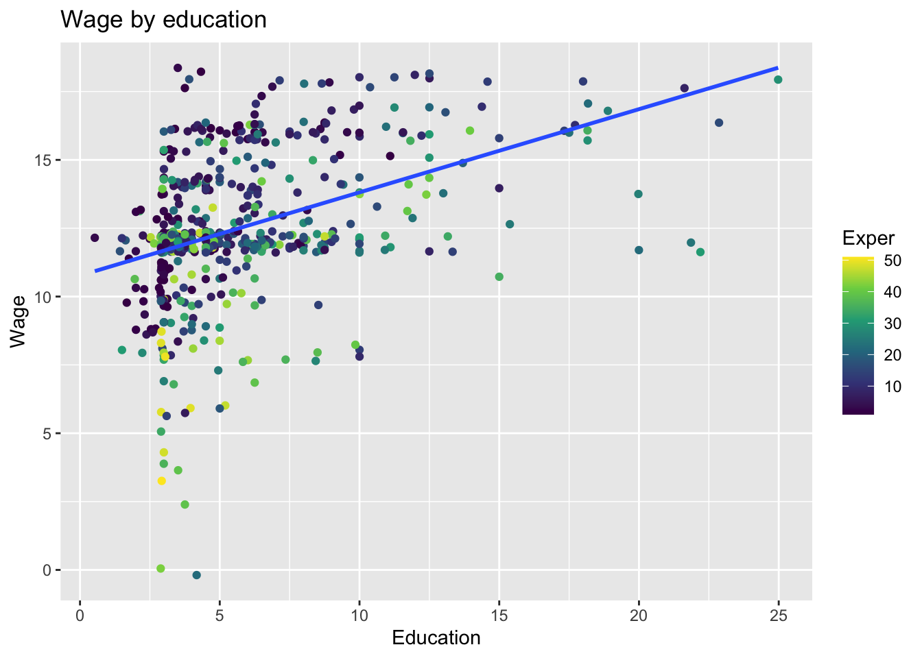

---

14.7 Additional practice questions

There’s an old saying (often attributed to Winston Churchill) that says, “If you are not a liberal when you are young, you have no heart. If you are not a conservative when you are old, you have no brain.” And, yet there have been activist left-wing groups comprised of seniors, like the Raging Grannies.

Using our sample CES dataset, explore the relationship between Canadians’ support for free market principles ($marketlib$) and age ($age$)? Is there is a relationship? If so, is it linear?

We’re going to run two regression models. Model 1 will regress $marketlib$ on $age$, while controlling for $gender$. Model 2 will be the same as Model 1, except it will also include the quadratic term for $age$ (i.e. $ag{e}^2$).

load("Sample_data/ces.rda")

Before we begin, it’s useful to look at the univariate distributions of out variables. Besides letting us know of missing values, it also helps with interpreting the substantive significance of any relationships we find.

summary(ces$marketlib)

##    Min. 1st Qu.  Median    Mean 3rd Qu.    Max.    NA's 
##    0.00    6.00    9.00    8.59   11.00   16.00   32684

sd(ces$marketlib, na.rm = TRUE)

## [1] 3.519915

summary(ces$age)

##    Min. 1st Qu.  Median    Mean 3rd Qu.    Max. 
##    18.0    35.0    49.0    48.7    62.0    99.0

sd(ces$age, na.rm = TRUE)

## [1] 16.60883

summary(ces$gender)

##   Man Woman  NA's 
## 15517 21928   288

table(ces$gender) %>% prop.table()

## 
##       Man     Woman 
## 0.4143944 0.5856056

Market liberalism variable ranges from 0 to 16, with a mean of 8.59 (SD = 3.52). (Note: this is a simple additive index, or summated rating scale, of four Likert-type items that has been commonly used in Canadian political science research.)

Age ranges from 18 to 99, with a mean of 49.0 (SD = 16.61).

Gender is categorical variable, with about 58.6% being women and 41.4% being men.

14.7.1 1. For both Model 1 and Model 2, write the equation of the population models.

Our population models are:

$$\begin{array}{rlrl}marketlib& ={\beta }_0+{\beta }_{1}gender+{\beta }_{2}age+\mu & & \text{(Model 1)}\\ marketlib& ={\beta }_0+{\beta }_{1}gender+{\beta }_{2}age+{\beta }_{3}ag{e}^2+\mu & & \text{(Model 2)}\end{array}$$

14.7.2 2. Run the regressions and write out the equations for the estimated regression models.

marketmod1 <- lm(marketlib ~ gender + age, data = ces)
summary(marketmod1)

## 
## Call:
## lm(formula = marketlib ~ gender + age, data = ces)
## 
## Residuals:
##     Min      1Q  Median      3Q     Max 
## -9.3775 -2.2386  0.2442  2.5586  8.2885 
## 
## Coefficients:
##              Estimate Std. Error t value Pr(>|t|)    
## (Intercept)  8.309741   0.195029  42.608  < 2e-16 ***
## genderWoman -0.855020   0.099390  -8.603  < 2e-16 ***
## age          0.013516   0.003192   4.234 2.34e-05 ***
## ---
## Signif. codes:  0 '***' 0.001 '**' 0.01 '*' 0.05 '.' 0.1 ' ' 1
## 
## Residual standard error: 3.474 on 5022 degrees of freedom
##   (32708 observations deleted due to missingness)
## Multiple R-squared:  0.02078,    Adjusted R-squared:  0.02039 
## F-statistic: 53.28 on 2 and 5022 DF,  p-value: < 2.2e-16

Our regression equation for Model 1 is:

$$\widehat{marketlib}=8.309-0.855gender+0.014age$$ $$\begin{gathered} n=5025 \\ {R}^2=0.021 \end{gathered}$$

marketmod2 <- lm(marketlib ~ gender + age + I(age^2), data = ces)
summary(marketmod2)

## 
## Call:
## lm(formula = marketlib ~ gender + age + I(age^2), data = ces)
## 
## Residuals:
##     Min      1Q  Median      3Q     Max 
## -9.2733 -2.2700  0.4905  2.5909  8.9988 
## 
## Coefficients:
##               Estimate Std. Error t value Pr(>|t|)    
## (Intercept)  6.2610833  0.5002976  12.515  < 2e-16 ***
## genderWoman -0.8560525  0.0992055  -8.629  < 2e-16 ***
## age          0.0996610  0.0196397   5.074 4.03e-07 ***
## I(age^2)    -0.0008238  0.0001853  -4.445 8.97e-06 ***
## ---
## Signif. codes:  0 '***' 0.001 '**' 0.01 '*' 0.05 '.' 0.1 ' ' 1
## 
## Residual standard error: 3.467 on 5021 degrees of freedom
##   (32708 observations deleted due to missingness)
## Multiple R-squared:  0.02461,    Adjusted R-squared:  0.02403 
## F-statistic: 42.24 on 3 and 5021 DF,  p-value: < 2.2e-16

Our regression equation for Model 2 is:

$$\widehat{marketlib}=6.261-0.856gender+0.100age-0.000824ag{e}^2$$ $$\begin{gathered} n=5025 \\ {R}^2=0.025 \end{gathered}$$

14.7.3 3. Explain what the coefficients mean in both models. How does the effect of age differ between Model 1 and Model 2?

Model 1, our coefficients are:

• $\widehat{{\beta }_0}$: This is the intercept, or the average predicted market liberalism score for men and those 0 years old. While the value is 7.966, this value is not theoretically meaningful.
• ${\hat{\beta }}_{age}$: For every additional year of age, we would predict a Canadian, on average, to be 0.022 more supportive of free market principles, holding all other things constant. With continuous variables like age, it’s often useful to convert the units–for example, we could represent this same relationship by saying that, on average, every increase of 10 years in age is associated with an increase of 0.220 on the market liberalism scale. (This also makes theoretical sense for a variable like age where we wouldn’t really expect a huge change year-over-year, but we might expect that for a change over 10 years.)
• ${\hat{\beta }}_{gender}$: Ceteris paribus, women score an average of 0.826 points lower than men on the market liberalism scale.

Model 2, our coefficients are:

• $\widehat{{\beta }_0}$: This is the intercept, or the average predicted market liberalism score for men and those 0 years old. While the value is 6.782, this value is not theoretically meaningful.
• ${\hat{\beta }}_{age}$ and ${\hat{\beta }}_{ag{e}^2}$: To understand the effect of age, we cannot just look at the coefficients for $age$ and $ag{e}^2$ individually; we have to look at them together. So, the effect of age on market liberalism is $0.77age-0.000569ag{e}^2$. This is non-linear, meaning the rate of change is not the same across all possible changes across values of age. It also might be non-monotonic, meaning it is positive for some changes across values fo age and negative for others. (If you want to see how we could graph this—which you don’t have to know for Assignment #1—it’s after Q4.)
• ${\hat{\beta }}_{gender}$: Ceteris paribus, women score an average of 0.827 points lower than men on the market liberalism scale.

14.7.4 4. Which of the models better explains the relationship between $marketlib$ and $age$?

The $R^2$ for Model 1 is 0.074 and for Model 2, it is 0.079. This suggests that Model 2 fits the data better than Model 1. There is a bit more to comparing model fit, and we’ll get to that in a few weeks time, but this is the starting point.

Also, empirical performance isn’t everything. Fortunately, there are also theoretical reasons to suspect that the effect of age might not be a clear-cut linear relationship suggested by the old adage. Older folks typically have lower levels of income and tend to rely upon the welfare state more than younger folks (on average, and all other things being equal). So, life-cycle effects might cause their interests to change, and by extension, their orientations on how society ought to be run.

There is also the issue that comparing across ages at one point in time cannot separate life-cycle effects from generational effects, which neither of these models would be able to disentangle.