6 Lecture 3: Core Concepts of Experimental Design

Slides

• 4 Core Concepts of Experimental Design (link)

6.1 Introduction

In this lecture we look at a (slightly) more technical understanding of selection bias (to understand the problem with observational data) and the potential outcomes approach (to understand how random assignment solves this problem).

The lecture slide are displayed in full below:

Figure 6.1: Slides for 4 Core Concepts of Experimental Design.

6.2 Vignette 3.1

Liebman, Jeffrey B., and Erzo FP Luttmer. “Would people behave differently if they better understood social security? Evidence from a field experiment.” American Economic Journal: Economic Policy 7.1 (2015): 275-99.

library(tidyverse) # for wrangling data
library(tidylog) # to know what we are wrangling
library(sjPlot) # to plot somse models
library(readstata13) # to load .dta files

exp_data <- read.dta13("Sample_data/Data_WithAgeInconsistency.dta")

Our variable of interest (DV, Y) is paid_work_yes: whether the person worked or not. Our treatment variable is treat: whether they got the pamphlet or not. Because this is an experiment, we can compare the averages of the treatment group and the control group to estimate the causal effect.

exp_data %>%
  group_by(treat) %>% 
  summarise(ATE = mean(paid_work_yes, na.rm = T))

## group_by: one grouping variable (treat)
## summarise: now 2 rows and 2 columns, ungrouped

## # A tibble: 2 × 2
##   treat   ATE
##   <dbl> <dbl>
## 1     0 0.744
## 2     1 0.785

Same effect as reported by authors!! We can also estimate differences by gender (why?):

exp_data %>%
  group_by(female,treat) %>% 
  summarise(ATE = mean(paid_work_yes, na.rm = T))

## group_by: 2 grouping variables (female, treat)
## summarise: now 4 rows and 3 columns, one group variable remaining (female)

## # A tibble: 4 × 3
## # Groups:   female [2]
##   female treat   ATE
##    <int> <dbl> <dbl>
## 1      0     0 0.784
## 2      0     1 0.787
## 3      1     0 0.713
## 4      1     1 0.782

Treatment only has an effect on women… why?

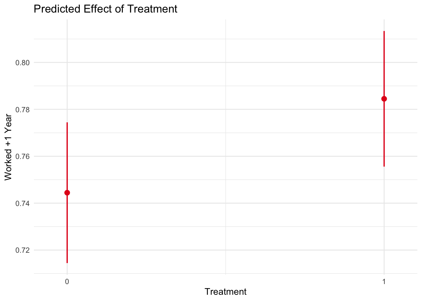
These averages look great and all but how can we be sure if these effects are not only a mere coincidence product of randomization? Let’s add some confidence intervals:

exp_data$treat <- as.factor(exp_data$treat)
exp_data$female <- as.factor(exp_data$female)

# Full model
model_1 <- lm(paid_work_yes ~ treat, data = exp_data)
summary(model_1)

## 
## Call:
## lm(formula = paid_work_yes ~ treat, data = exp_data)
## 
## Residuals:
##     Min      1Q  Median      3Q     Max 
## -0.7845  0.2155  0.2155  0.2555  0.2555 
## 
## Coefficients:
##             Estimate Std. Error t value Pr(>|t|)    
## (Intercept)  0.74446    0.01530  48.666   <2e-16 ***
## treat1       0.04004    0.02124   1.885   0.0596 .  
## ---
## Signif. codes:  0 '***' 0.001 '**' 0.01 '*' 0.05 '.' 0.1 ' ' 1
## 
## Residual standard error: 0.4237 on 1591 degrees of freedom
##   (890 observations deleted due to missingness)
## Multiple R-squared:  0.002228,   Adjusted R-squared:  0.001601 
## F-statistic: 3.553 on 1 and 1591 DF,  p-value: 0.05961

plot_model(model_1, type = "pred", terms = "treat") +
  theme_minimal() +
  labs(x="Treatment", y="Worked +1 Year",
       title="Predicted Effect of Treatment")

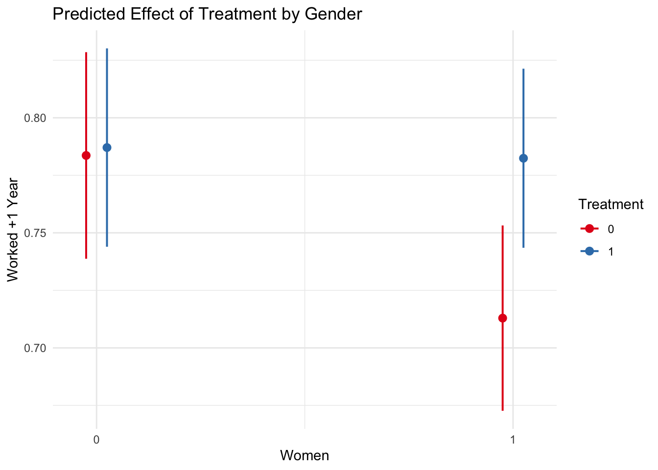
And now by gender:

# Model by gender
model_2 <- lm(paid_work_yes ~ female + treat + female*treat, data = exp_data)
summary(model_2)

## 
## Call:
## lm(formula = paid_work_yes ~ female + treat + female * treat, 
##     data = exp_data)
## 
## Residuals:
##     Min      1Q  Median      3Q     Max 
## -0.7871  0.2129  0.2164  0.2176  0.2871 
## 
## Coefficients:
##                 Estimate Std. Error t value Pr(>|t|)    
## (Intercept)     0.783626   0.022885  34.242   <2e-16 ***
## female1        -0.070685   0.030743  -2.299   0.0216 *  
## treat1          0.003436   0.031725   0.108   0.9138    
## female1:treat1  0.066040   0.042680   1.547   0.1220    
## ---
## Signif. codes:  0 '***' 0.001 '**' 0.01 '*' 0.05 '.' 0.1 ' ' 1
## 
## Residual standard error: 0.4232 on 1589 degrees of freedom
##   (890 observations deleted due to missingness)
## Multiple R-squared:  0.005552,   Adjusted R-squared:  0.003675 
## F-statistic: 2.957 on 3 and 1589 DF,  p-value: 0.03136

plot_model(model_2, type = "int") +
  theme_minimal() +
  labs(x="Women", y="Worked +1 Year", color = "Treatment",
       title="Predicted Effect of Treatment by Gender")

Cool…