3 Lecture 2: Introduction to Causal Inference
Slides
- 3 Introduction to Causal Inference (link)
3.1 Introduction
We now dive deeper into causal inference and the counterfactual problem. We show why randomized trials solve the counterfactual problem, but also why it remains a challenge when using observational data.
The lecture slides are displayed in full below:
Figure 3.1: Slides for 3 Introduction to Causal Inference.
3.2 Vignette 2.1
Usually, we do not know the data-generating process, but here, we are gods. Let’s create a world where taking treatment A (e.g., taking a pill) positively affects Y (e.g., health) by one unit. Let’s run an experiment.
df <- data.frame(health_no_pill= rnorm(5000),
                 # Randomly assign a treatment
                 pill=sample(c(0,1),5000,replace=T))
hist(df$health_no_pill)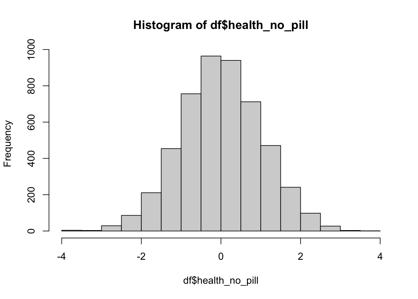
| Var1 | Freq |
|---|---|
| 0 | 2514 |
| 1 | 2486 |
Now we can create our counterfactual:
df <- df %>%
  mutate(health_w_pill = health_no_pill + 1) # Our Y when A=1 aka our counterfactual
## mutate: new variable
## 'health_w_pill' (double) with
## 5,000 unique values and 0% NALet’s look at our counterfactual:
health_w_pill <- cbind.data.frame(df$health_w_pill,"with Pill")
colnames(health_w_pill) <- c("health","treatment")
health_no_pill <- cbind.data.frame(df$health_no_pill,"without Pill")
colnames(health_no_pill) <- c("health","treatment")
comparison_y <- rbind.data.frame(health_w_pill,health_no_pill)

comparison_y %>%
  group_by(treatment) %>%
  mutate(mean_health = mean(health)) %>%
  ungroup() %>%
  ggplot(aes(x=health,fill = treatment,color = treatment)) +
  geom_density(alpha = .5) +
  scale_x_continuous(breaks = scales::pretty_breaks(n = 8)) +
  geom_vline(aes(xintercept = mean_health, color = treatment ),
             linetype = "dashed")
## group_by: one grouping variable (treatment)
## mutate (grouped): new variable 'mean_health' (double) with 2 unique values and 0% NA
## ungroup: no grouping variables remain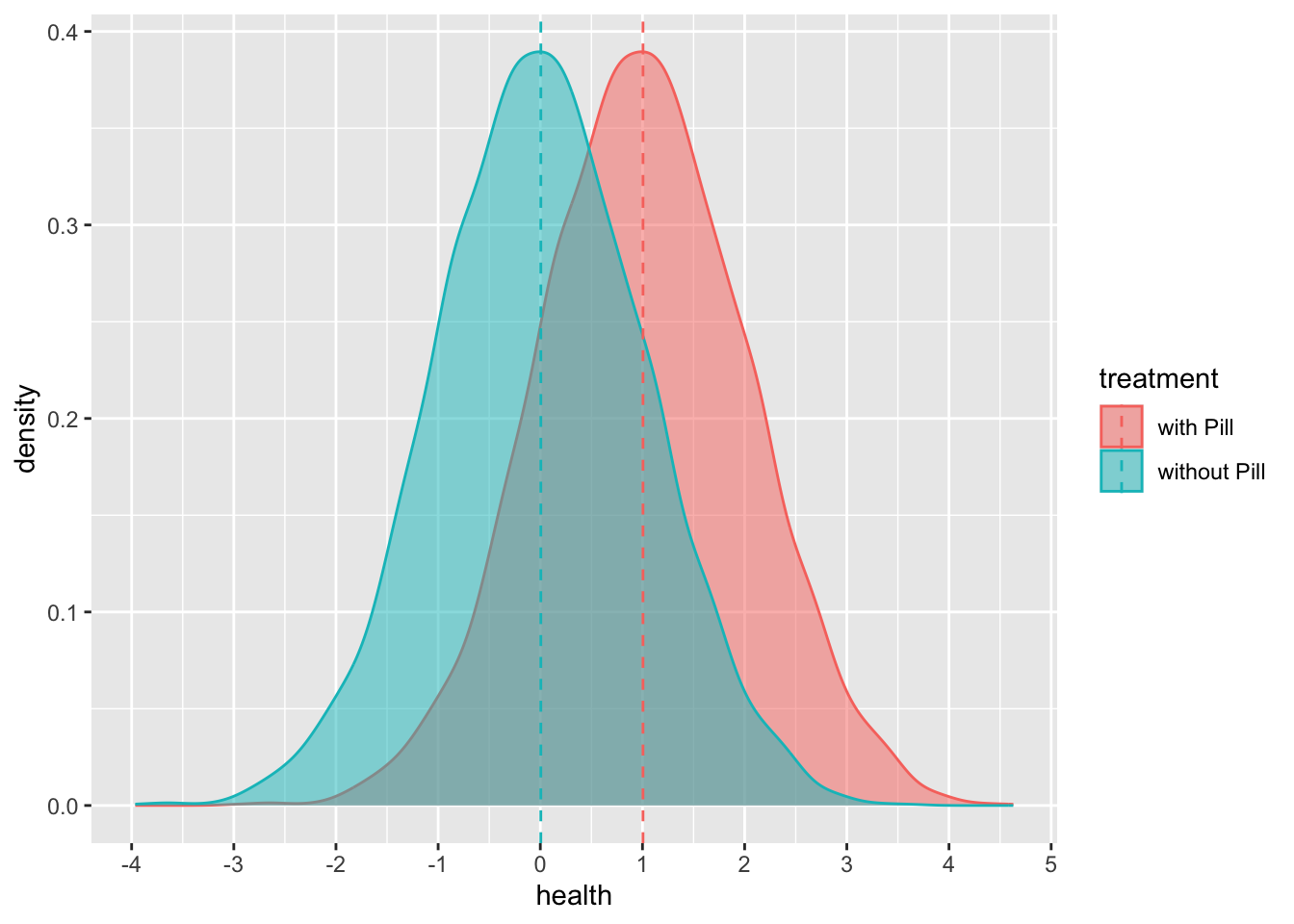
Now let’s give each individual the treatment (either the pill or a placebo):
## mutate: new variable
## 'health_obs' (double) with
## 5,000 unique values and 0% NA
head(df,10)## health_no_pill pill
## 1 -0.74805710 1
## 2 -1.81223474 1
## 3 -1.60532597 1
## 4 1.61295877 0
## 5 0.73325187 1
## 6 0.61742920 0
## 7 -0.54035594 1
## 8 0.04804552 0
## 9 1.45788206 1
## 10 -0.81084986 1
## health_w_pill health_obs
## 1 0.2519429 0.25194290
## 2 -0.8122347 -0.81223474
## 3 -0.6053260 -0.60532597
## 4 2.6129588 1.61295877
## 5 1.7332519 1.73325187
## 6 1.6174292 0.61742920
## 7 0.4596441 0.45964406
## 8 1.0480455 0.04804552
## 9 2.4578821 2.45788206
## 10 0.1891501 0.18915014We can see the average effect of the pill on the treated group (remember from the lecture that the effect is, in essence, the difference between those who receive the treatment and those who do not):
## group_by: one grouping variable (pill)
## summarize: now 2 rows and 2 columns, ungrouped
## # A tibble: 2 × 2
## pill health
## <dbl> <dbl>
## 1 0 -0.000254
## 2 1 1.02Or we can plot it:
df %>%
  group_by(pill) %>%
  mutate(mean_health_obs = mean(health_obs)) %>%
  ungroup() %>%
  ggplot(aes(x=health_obs,fill = factor(pill),color = factor(pill))) +
  geom_density(alpha = .5) +
  scale_x_continuous(breaks = scales::pretty_breaks(n = 8)) +
  geom_vline(aes(xintercept = mean_health_obs, color = factor(pill) ),
             linetype = "dashed")
## group_by: one grouping variable (pill)
## mutate (grouped): new variable 'mean_health_obs' (double) with 2 unique values and 0% NA
## ungroup: no grouping variables remain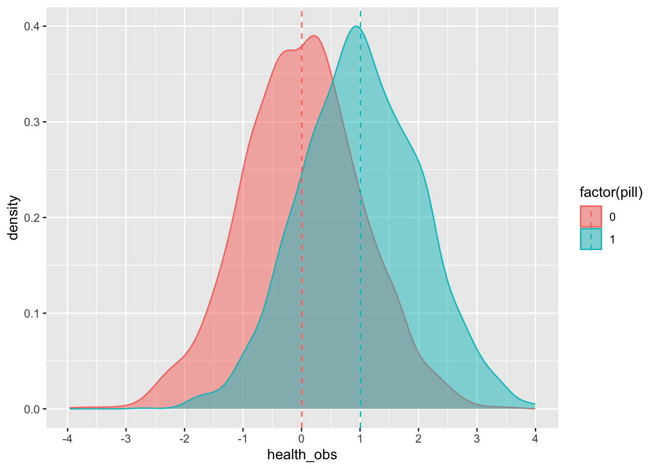
3.3 Vignette 2.2
Ok… but what happens if we cannot randomize? What if we have observational data, such that…
df <- data.frame(income = runif(10000)) %>%
  # In this case, your health is determined randomly AND by your levels of income
  mutate(health_no_pill = rnorm(10000) + income,
         health_w_pill = health_no_pill + 1) %>%
  # Now we give the pill only to people that have money
  mutate(pill = income > .7,
         health_obs = ifelse(pill==1,health_w_pill,health_no_pill))
## mutate: new variable 'health_no_pill' (double) with 10,000 unique values and 0% NA
## new variable 'health_w_pill' (double) with 10,000 unique values and 0% NA
## mutate: new variable 'pill' (logical) with 2 unique values and 0% NA
## new variable 'health_obs' (double) with 10,000 unique values and 0% NA
head(df,10)## income health_no_pill
## 1 0.53220279 0.1884822
## 2 0.48299455 3.0202510
## 3 0.28378160 -0.9988499
## 4 0.69812081 -0.1399785
## 5 0.39569507 0.3731290
## 6 0.93720899 1.2019669
## 7 0.84051199 0.1108285
## 8 0.02931242 1.5006180
## 9 0.35096344 0.7021132
## 10 0.65176919 0.7508874
## health_w_pill pill
## 1 1.188482185 FALSE
## 2 4.020251017 FALSE
## 3 0.001150149 FALSE
## 4 0.860021501 FALSE
## 5 1.373128951 FALSE
## 6 2.201966949 TRUE
## 7 1.110828494 TRUE
## 8 2.500618039 FALSE
## 9 1.702113170 FALSE
## 10 1.750887357 FALSE
## health_obs
## 1 0.1884822
## 2 3.0202510
## 3 -0.9988499
## 4 -0.1399785
## 5 0.3731290
## 6 2.2019669
## 7 1.1108285
## 8 1.5006180
## 9 0.7021132
## 10 0.7508874Let’s see what happens now to the estimated mean average ‘effect’ (remember from the lecture that the effect is, in essence, the difference between those who receive the treatment and those who do not):
## group_by: one grouping variable (pill)
## summarize: now 2 rows and 2 columns, ungrouped
## # A tibble: 2 × 2
## pill health
## <lgl> <dbl>
## 1 FALSE 0.367
## 2 TRUE 1.81Oh no! That is more than the actual effect of the pill, which we know is 1 since we created it. However, if we were to properly model (this is an RDD!), then (remember from the lecture that the effect is, in essence, the difference between those who receive the treatment, and those who do not):
df %>%
  filter(abs(income-.7)<.01) %>%
  group_by(pill) %>%
  summarize(health = mean(health_obs)) ## BOOM!!
## filter: removed 9,777 rows (98%), 223 rows remaining
## group_by: one grouping variable (pill)
## summarize: now 2 rows and 2 columns, ungrouped## # A tibble: 2 × 2
## pill health
## <lgl> <dbl>
## 1 FALSE 0.693
## 2 TRUE 1.72