15 Lecture 6: The Multiple Regression Model I

Slides

• 7 The Multiple Regression Model (link)

15.1 Introduction

## 
## Attaching package: 'ggpubr'

## The following objects are masked from 'package:tidylog':
## 
##     group_by, mutate

We continue studying the simple regression model.

Figure 15.1: Slides for 7 The Multiple Regression Model.

15.2 Vignette 6.1

Once again, let’s simulate some data. Maybe we are interested in urban and rural towns (70% are urban) :

df <- tibble(urban = sample(c(0,1),500,replace=T,prob=c(.3,.7))) %>%
  ## Urban towns spend, on average, $3 million more on wages than rural towns
  mutate(expen_wages = 3*urban+runif(500,min=0,max=4)) %>%
  ## Urban towns are also have greater incomes (e.g., from taxes), but these are reduced by their high wage expenditures:
  mutate(log_income = 1 + 2*urban - .3*expen_wages + rnorm(500,mean=2)) ## <- Population Eq.

Now we can estimate the effect of wage expenditure on income:

model_a <- lm(log_income ~ expen_wages, data = df) 
summary(model_a) 

## 
## Call:
## lm(formula = log_income ~ expen_wages, data = df)
## 
## Residuals:
##     Min      1Q  Median 
## -3.9713 -0.7411  0.0280 
##      3Q     Max 
##  0.7812  2.9860 
## 
## Coefficients:
##             Estimate
## (Intercept)  2.98686
## expen_wages  0.06318
##             Std. Error t value
## (Intercept)    0.11844  25.219
## expen_wages    0.02663   2.373
##             Pr(>|t|)    
## (Intercept)   <2e-16 ***
## expen_wages    0.018 *  
## ---
## Signif. codes:  
##   0 '***' 0.001 '**' 0.01
##   '*' 0.05 '.' 0.1 ' ' 1
## 
## Residual standard error: 1.142 on 498 degrees of freedom
## Multiple R-squared:  0.01118,    Adjusted R-squared:  0.009194 
## F-statistic: 5.631 on 1 and 498 DF,  p-value: 0.01803

Wait what? (Interpret a log ~ level)

15.3 Vignette 6.2

Let’s see… How can we remove everything from wages that is explained by urban? How can we remove everything from income that is explained by urban?

df %>% group_by(urban) %>%
  summarise(income_urb= mean(log_income)) 

## summarise: now 2 rows and 2
## columns, ungrouped

## # A tibble: 2 × 2
##   urban income_urb
##   <dbl>      <dbl>
## 1     0       2.60
## 2     1       3.52

df %>% group_by(urban) %>% 
  summarise(expen_wages_urb = mean(expen_wages))

## summarise: now 2 rows and 2
## columns, ungrouped

## # A tibble: 2 × 2
##   urban expen_wages_urb
##   <dbl>           <dbl>
## 1     0            1.72
## 2     1            5.03

The difference between what is explained by urban of income/expendinture (mean) and the observed value of income/expenditure is…

df <- df %>% group_by(urban) %>%
  mutate(log_income_residual = log_income - mean(log_income),
         expen_wages_residual = expen_wages - mean(expen_wages)) %>%
  ungroup()

## ungroup: no grouping variables
## remain

The residual… what is not explained by urban!!

model_b <- lm(log_income_residual ~ expen_wages_residual, data = df) 
summary(model_b) ### CLOSER!

## 
## Call:
## lm(formula = log_income_residual ~ expen_wages_residual, data = df)
## 
## Residuals:
##     Min      1Q  Median 
## -3.5403 -0.7092  0.0195 
##      3Q     Max 
##  0.7024  2.7306 
## 
## Coefficients:
##                        Estimate
## (Intercept)          -1.621e-16
## expen_wages_residual -3.039e-01
##                      Std. Error
## (Intercept)           4.502e-02
## expen_wages_residual  3.868e-02
##                      t value
## (Intercept)            0.000
## expen_wages_residual  -7.857
##                      Pr(>|t|)
## (Intercept)                 1
## expen_wages_residual 2.44e-14
##                         
## (Intercept)             
## expen_wages_residual ***
## ---
## Signif. codes:  
##   0 '***' 0.001 '**' 0.01
##   '*' 0.05 '.' 0.1 ' ' 1
## 
## Residual standard error: 1.007 on 498 degrees of freedom
## Multiple R-squared:  0.1103, Adjusted R-squared:  0.1085 
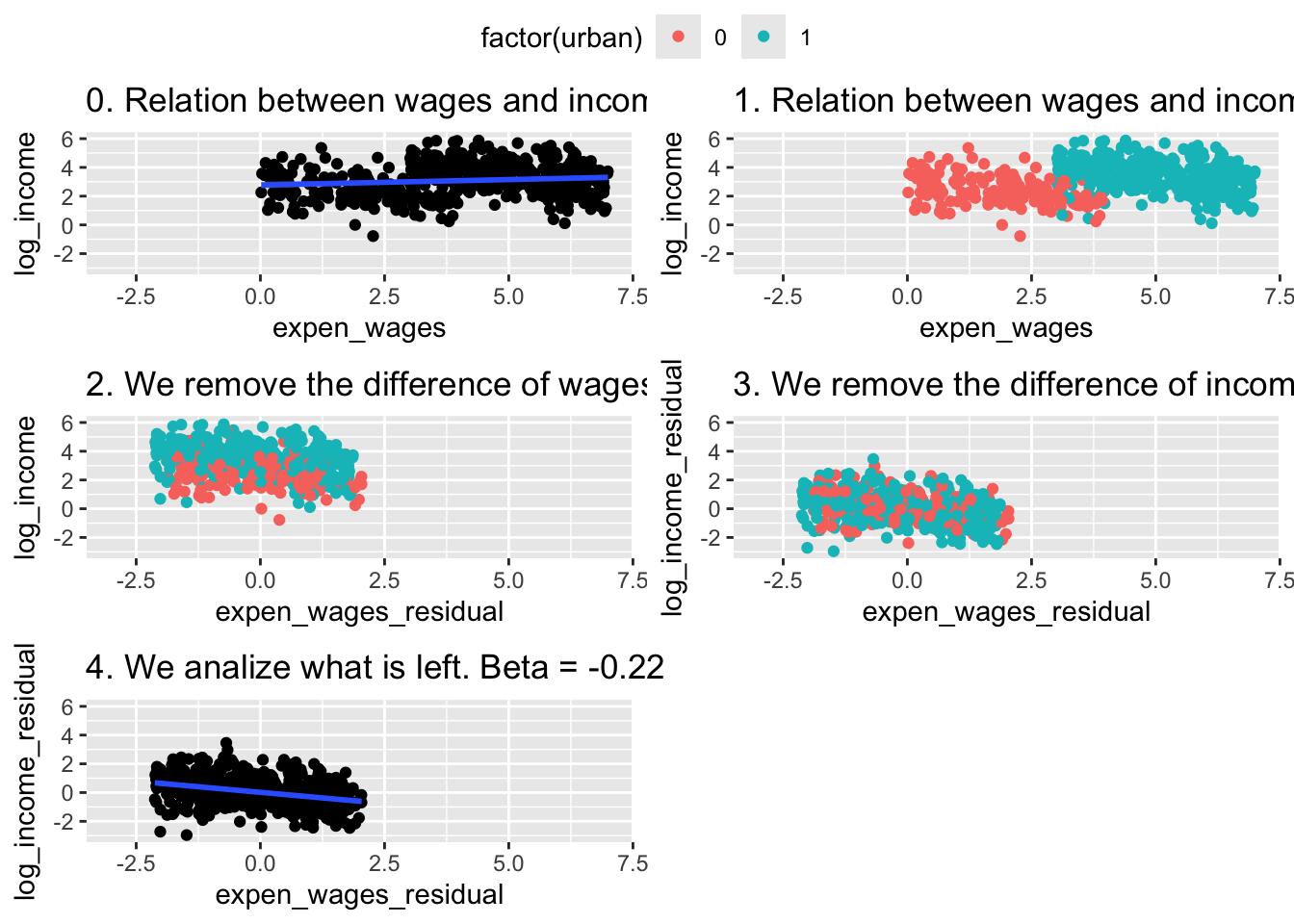
## F-statistic: 61.73 on 1 and 498 DF,  p-value: 2.444e-14

Let’s plot:

A <- ggplot(df, aes(x=expen_wages,y=log_income)) +
  geom_point() +
  labs(title = "0. Relation between wages and income. Beta = 0.13") +
  geom_smooth(method = "lm") +
  xlim(c(-3,7)) + ylim(c(-3,6))
A

## `geom_smooth()` using formula
## = 'y ~ x'

B <- ggplot(df, aes(x=expen_wages,y=log_income,color = factor(urban))) +
  geom_point() +
  labs(title = "1. Relation between wages and income divided by urban.") +
  xlim(c(-3,7)) + ylim(c(-3,6))
B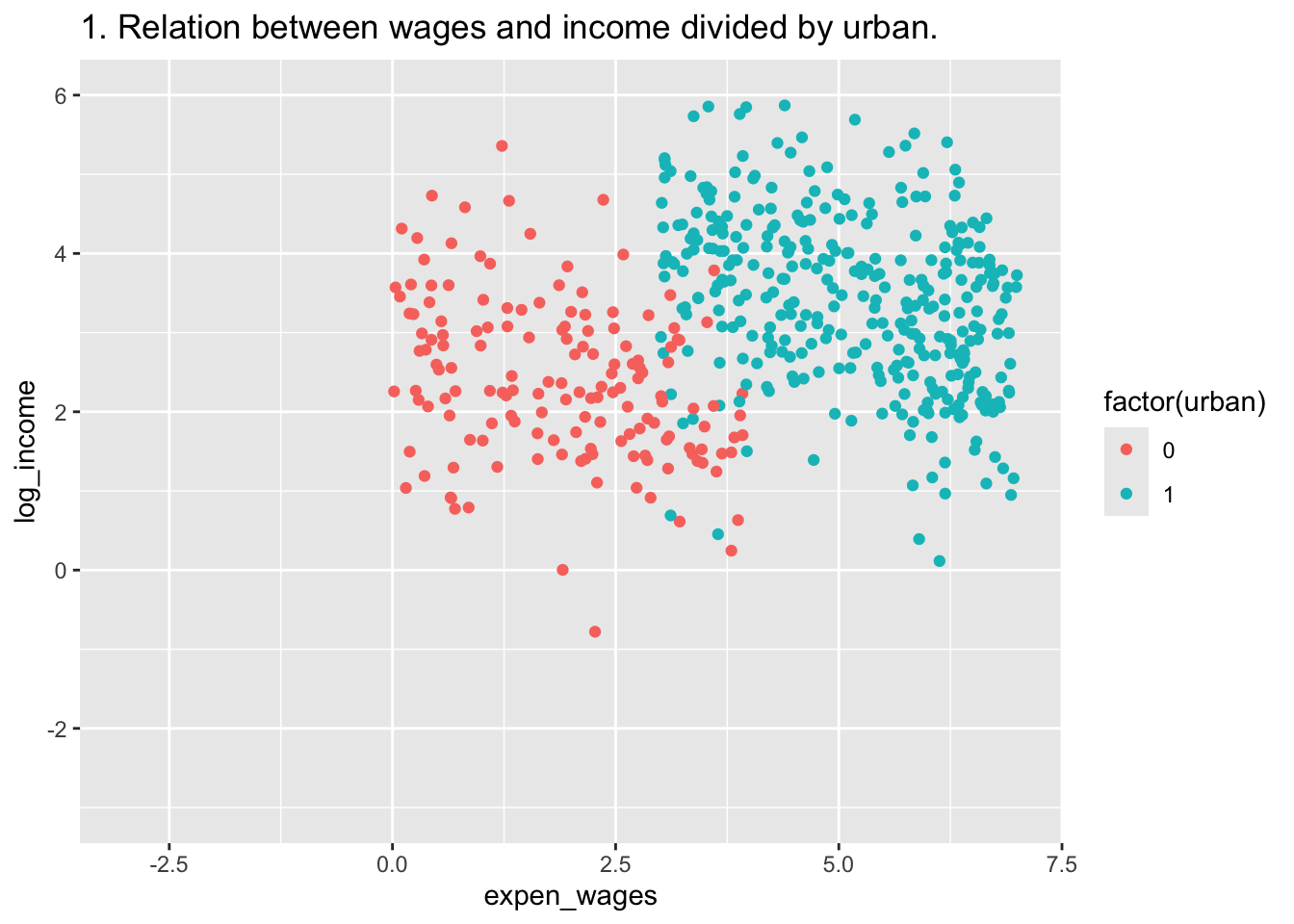

C <- ggplot(df, aes(x=expen_wages_residual,y=log_income,color = factor(urban))) +
  geom_point() +
  labs(title = "2. We remove the difference of wages explained by urban.")+
  xlim(c(-3,7)) + ylim(c(-3,6))
C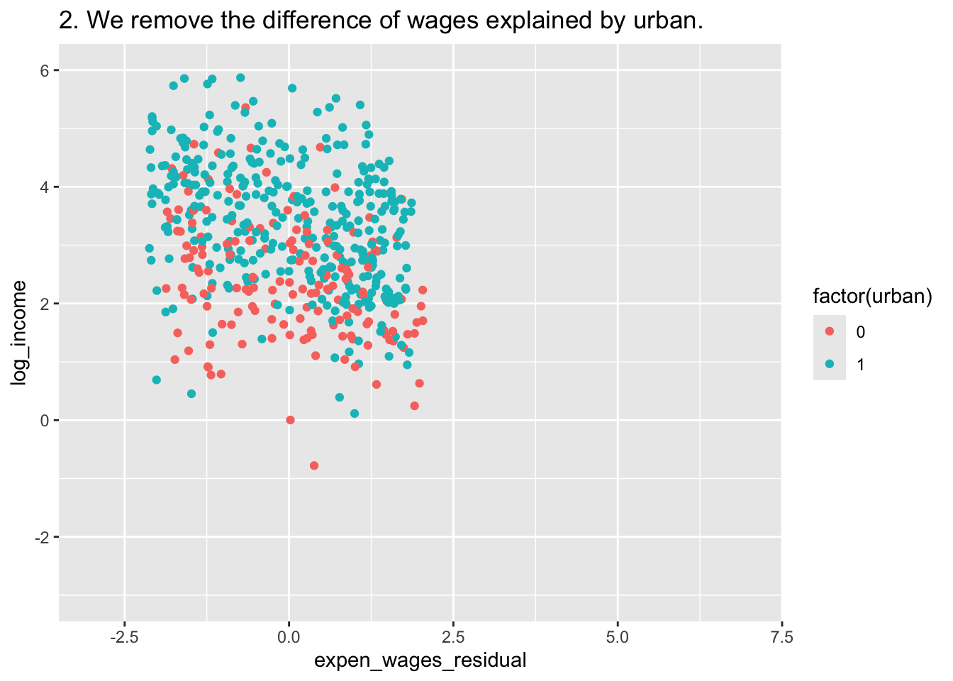

D <- ggplot(df, aes(x=expen_wages_residual,y=log_income_residual,color = factor(urban))) +
  geom_point() +
  labs(title = "3. We remove the difference of income explained by urban.")+
  xlim(c(-3,7)) + ylim(c(-3,6))
D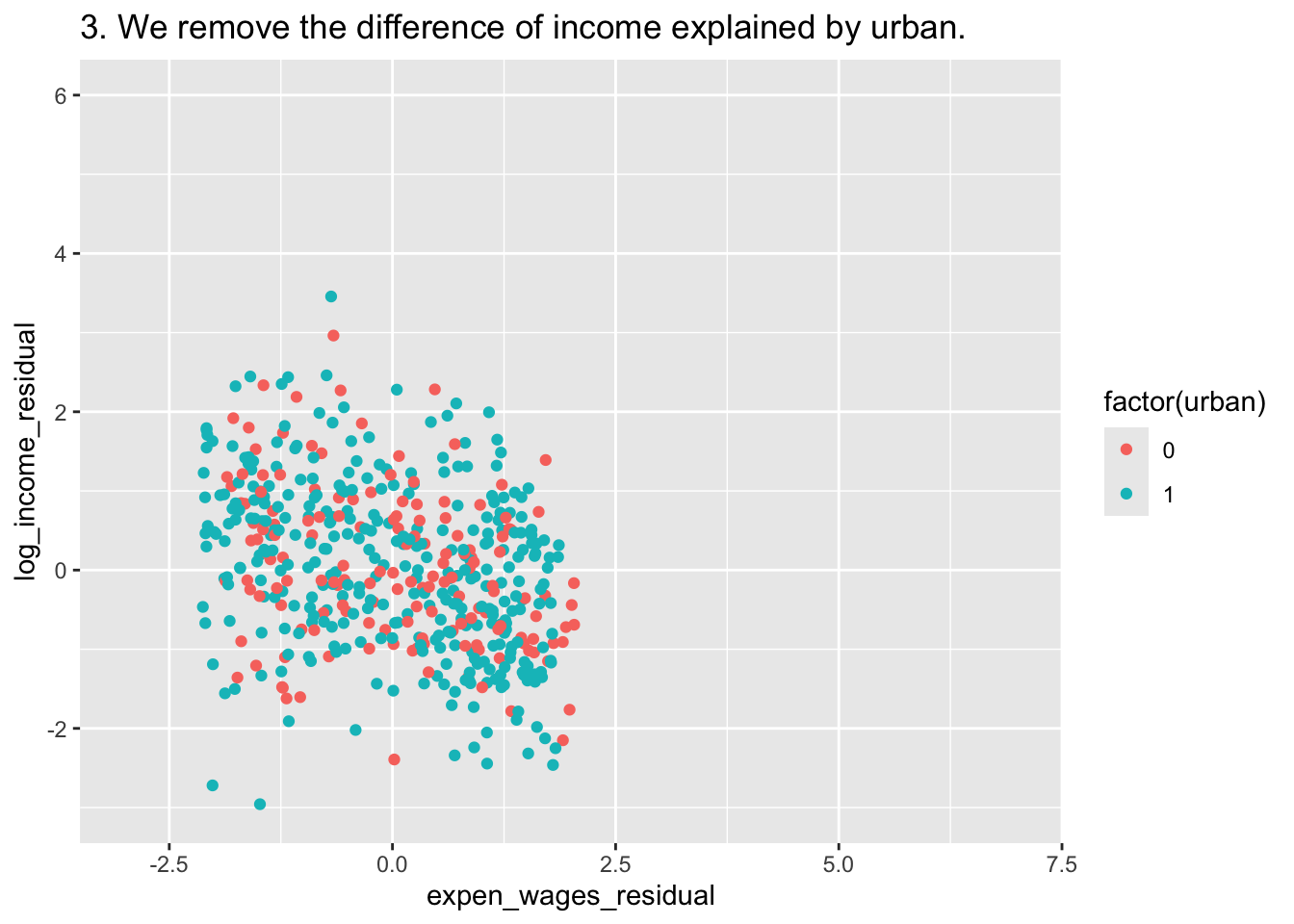

E <- ggplot(df, aes(expen_wages_residual,y=log_income_residual)) +
  geom_point() +
  labs(title = "4. We analize what is left. Beta = -0.22") +
  geom_smooth(method = "lm")+
  xlim(c(-3,7)) + ylim(c(-3,6))
E

## `geom_smooth()` using formula
## = 'y ~ x'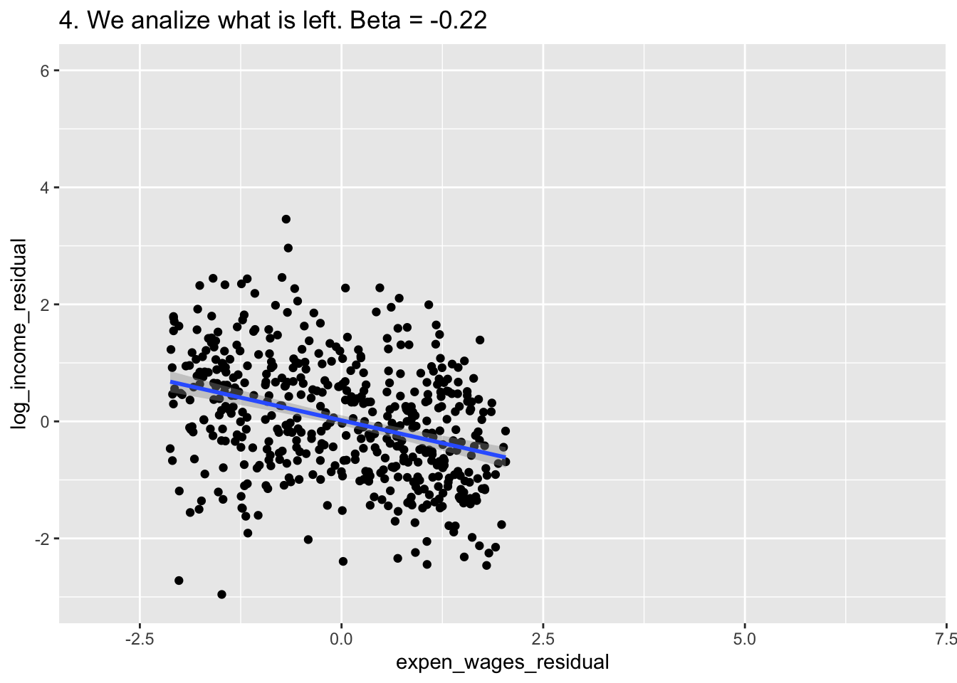

ggarrange(A,B,C,D,E,
          common.legend = T,
          ncol = 2,
          nrow = 3)

## `geom_smooth()` using formula
## = 'y ~ x'
## `geom_smooth()` using formula
## = 'y ~ x'
## `geom_smooth()` using formula
## = 'y ~ x'