21 Lecture 9 Exercises
This tutorial was created by John Santos (with minor adaptations from me). This tutorial covers carrying out hypothesis testing in R.
library(tidyverse)
library(car)
load("Sample_data/ces.rda")
mod <- lm(feel_cpc ~ woman + age + univ +
            marketlib + moraltrad, data = ces)
summary(mod)
##
## Call:
## lm(formula = feel_cpc ~ woman + age + univ + marketlib + moraltrad,
## data = ces)
##
## Residuals:
## Min 1Q Median 3Q Max
## -79.594 -22.510 -0.289 22.511 86.068
##
## Coefficients:
## Estimate Std. Error t value Pr(>|t|)
## (Intercept) 5.67469 3.00978 1.885 0.059496 .
## woman -4.53724 1.24012 -3.659 0.000259 ***
## age -0.02066 0.03947 -0.524 0.600618
## univ 0.50494 1.26471 0.399 0.689739
## marketlib 2.71180 0.18729 14.479 < 2e-16 ***
## moraltrad 2.83293 0.18193 15.572 < 2e-16 ***
## ---
## Signif. codes: 0 '***' 0.001 '**' 0.01 '*' 0.05 '.' 0.1 ' ' 1
##
## Residual standard error: 29.49 on 2375 degrees of freedom
## (35352 observations deleted due to missingness)
## Multiple R-squared: 0.2596, Adjusted R-squared: 0.2581
## F-statistic: 166.6 on 5 and 2375 DF, p-value: < 2.2e-16
21.1 The {car} package and the functions linearHypothesis() and Anova()
(Not to be confused with Base R’s anova())
While you will learn how to conduct hypothesis testing manually using re-parameterized models, in practice, we often use pre-programmed functions, such as the linearHypothesis() function from the car package.
For our purposes, it takes two arguments:
-
object= our model object (in this case,mod) - the hypothesis or hypotheses to be tested in quotes (in the following case,
"marketlib = 0") - note: multiple hypotheses can be tested if they are enclosed in separate quoted equations and combined with the
c()command (e.g.c("age = 0", "univ = 0"))
21.1.1 A basic test of one term’s statistical significance, e.g. is marketlib != 0?
We would never use this because we could just look at the summary table, but it does work.
This is also useful to show that F-tests and t-tests sort of do the same thing, but in different ways. The tests in the model summary table are t-tests of a term against 0, so they return t-statistics. linearHypothesis() uses an F-test, so it returns F-statistics.
But, you can see the F-statistics and t-statistics return the same p-values.
library(car)

linearHypothesis(mod, "marketlib=0")
##
## Linear hypothesis test:
## marketlib = 0
##
## Model 1: restricted model
## Model 2: feel_cpc ~ woman + age + univ + marketlib + moraltrad
##
## Res.Df RSS Df Sum of Sq F Pr(>F)
## 1 2376 2247929
## 2 2375 2065588 1 182341 209.65 < 2.2e-16 ***
## ---
## Signif. codes: 0 '***' 0.001 '**' 0.01 '*' 0.05 '.' 0.1 ' ' 1
linearHypothesis(mod, "marketlib=0") %>% as_tibble()## # A tibble: 2 × 6
## Res.Df RSS Df `Sum of Sq` F `Pr(>F)`
## <dbl> <dbl> <dbl> <dbl> <dbl> <dbl>
## 1 2376 2247929. NA NA NA NA
## 2 2375 2065588. 1 182341. 210. 1.35e-45
summary(mod)$coefficients ## Estimate Std. Error t value Pr(>|t|)
## (Intercept) 5.67469015 3.00978465 1.8854140 5.949593e-02
## woman -4.53724017 1.24012170 -3.6587056 2.590110e-04
## age -0.02066458 0.03946767 -0.5235825 6.006178e-01
## univ 0.50494416 1.26470847 0.3992574 6.897395e-01
## marketlib 2.71180033 0.18728635 14.4794339 1.349400e-45
## moraltrad 2.83292849 0.18192678 15.5718055 3.914799e-5221.1.2 Testing whether one term is different from another, e.g. is marketlib != moraltrad?
The effect of moraltrad is a about 0.1 larger than that of marketlib, but is this difference statistically significant?
linearHypothesis(mod, "marketlib = moraltrad")##
## Linear hypothesis test:
## marketlib - moraltrad = 0
##
## Model 1: restricted model
## Model 2: feel_cpc ~ woman + age + univ + marketlib + moraltrad
##
## Res.Df RSS Df Sum of Sq F Pr(>F)
## 1 2376 2065722
## 2 2375 2065588 1 133.82 0.1539 0.6949Notice how the linearHypothesis() function reformulates “marketlib != moraltrad” to “marketlib - moraltrad == 0” (just like a t-test).
linearHypothesis(mod, "marketlib - moraltrad = 0")##
## Linear hypothesis test:
## marketlib - moraltrad = 0
##
## Model 1: restricted model
## Model 2: feel_cpc ~ woman + age + univ + marketlib + moraltrad
##
## Res.Df RSS Df Sum of Sq F Pr(>F)
## 1 2376 2065722
## 2 2375 2065588 1 133.82 0.1539 0.694921.1.3 Testing the joint significance of multiple variables, e.g. “age and univ are jointly != 0”:
linearHypothesis(mod, c("age = 0", "univ = 0"))##
## Linear hypothesis test:
## age = 0
## univ = 0
##
## Model 1: restricted model
## Model 2: feel_cpc ~ woman + age + univ + marketlib + moraltrad
##
## Res.Df RSS Df Sum of Sq F Pr(>F)
## 1 2377 2066009
## 2 2375 2065588 2 420.89 0.242 0.785121.1.4 Testing if at least one term in the model is significant
This test asks if at least one of woman, age, univ, marketlib, or moraltrad is different from zero.
linearHypothesis(mod, c("woman = 0",
                        "age = 0",
                        "univ = 0",
                        "marketlib = 0",
                        "moraltrad = 0"))
##
## Linear hypothesis test:
## woman = 0
## age = 0
## univ = 0
## marketlib = 0
## moraltrad = 0
##
## Model 1: restricted model
## Model 2: feel_cpc ~ woman + age + univ + marketlib + moraltrad
##
## Res.Df RSS Df Sum of Sq F Pr(>F)
## 1 2380 2789889
## 2 2375 2065588 5 724301 166.56 < 2.2e-16 ***
## ---
## Signif. codes: 0 '***' 0.001 '**' 0.01 '*' 0.05 '.' 0.1 ' ' 1Note, this is the same as the F-test for the overall significance of a regression, which is reported in the model summary table.
summary(mod)##
## Call:
## lm(formula = feel_cpc ~ woman + age + univ + marketlib + moraltrad,
## data = ces)
##
## Residuals:
## Min 1Q Median 3Q Max
## -79.594 -22.510 -0.289 22.511 86.068
##
## Coefficients:
## Estimate Std. Error t value Pr(>|t|)
## (Intercept) 5.67469 3.00978 1.885 0.059496 .
## woman -4.53724 1.24012 -3.659 0.000259 ***
## age -0.02066 0.03947 -0.524 0.600618
## univ 0.50494 1.26471 0.399 0.689739
## marketlib 2.71180 0.18729 14.479 < 2e-16 ***
## moraltrad 2.83293 0.18193 15.572 < 2e-16 ***
## ---
## Signif. codes: 0 '***' 0.001 '**' 0.01 '*' 0.05 '.' 0.1 ' ' 1
##
## Residual standard error: 29.49 on 2375 degrees of freedom
## (35352 observations deleted due to missingness)
## Multiple R-squared: 0.2596, Adjusted R-squared: 0.2581
## F-statistic: 166.6 on 5 and 2375 DF, p-value: < 2.2e-16
21.2 Calculating p values of t statistics using R
We can also use R to calculate p values for a t test using the function pt().
Recall, the summary table for the model. I extract this manually because the printout from the summary() command rounds p values to 2e-16.
summary(mod)$coefficients## Estimate Std. Error t value Pr(>|t|)
## (Intercept) 5.67469015 3.00978465 1.8854140 5.949593e-02
## woman -4.53724017 1.24012170 -3.6587056 2.590110e-04
## age -0.02066458 0.03946767 -0.5235825 6.006178e-01
## univ 0.50494416 1.26470847 0.3992574 6.897395e-01
## marketlib 2.71180033 0.18728635 14.4794339 1.349400e-45
## moraltrad 2.83292849 0.18192678 15.5718055 3.914799e-52For a one-tailed test for marketlib >= 0…
## [1] 1For a one-tailed test for marketlib <= 0…
## [1] 6.747001e-46For a two-tailed test for marketlib = 0…
## [1] 1.3494e-4521.3 Confidence intervals
Recall, the formula for constructing a confidence interval is
\[CI_{\beta_j} = \hat{\beta}_j \pm (c \times se_{\hat{\beta}_j})\],
where \(c\) is the percentile in the \(t_{n-k-1}\) distribution that corresponds to our confidence interval. For the 90%, 95%, and 99% confidence intervals, this corresponds to, respectively, 1.64, 1.96, and 2.57.
So, if we wanted to build a CI around the coefficient for marketlib, we first have to pull up the table of coefficients
summary(mod)$coefficients## Estimate Std. Error t value Pr(>|t|)
## (Intercept) 5.67469015 3.00978465 1.8854140 5.949593e-02
## woman -4.53724017 1.24012170 -3.6587056 2.590110e-04
## age -0.02066458 0.03946767 -0.5235825 6.006178e-01
## univ 0.50494416 1.26470847 0.3992574 6.897395e-01
## marketlib 2.71180033 0.18728635 14.4794339 1.349400e-45
## moraltrad 2.83292849 0.18192678 15.5718055 3.914799e-52and note that the coefficient for marketlib is in [5,1] and the SE is in [5,2]
summary(mod)$coefficients[5,1]## [1] 2.7118
summary(mod)$coefficients[5,2]## [1] 0.1872864and then use the formula to calculate the lower bound
## [1] 2.344719and the upper bound.
## [1] 3.078882The above can be vectorized:
B + ( c(-1,1) * (1.96 * SE) )
## [1] 2.344719 3.078882You could also use tidyverse conventions to calculate all of the confidence intervals:
summary(mod)$coefficients %>%
  as.data.frame() %>%
  mutate(lower90 = Estimate - (`Std. Error` * 1.64),
         upper90 = Estimate + (`Std. Error` * 1.64),
         lower95 = Estimate - (`Std. Error` * 1.96),
         upper95 = Estimate + (`Std. Error` * 1.96),
         lower99 = Estimate - (`Std. Error` * 2.57),
         upper99 = Estimate + (`Std. Error` * 2.57))
## Estimate Std. Error t value Pr(>|t|) lower90
## (Intercept) 5.67469015 3.00978465 1.8854140 5.949593e-02 0.73864332
## woman -4.53724017 1.24012170 -3.6587056 2.590110e-04 -6.57103977
## age -0.02066458 0.03946767 -0.5235825 6.006178e-01 -0.08539156
## univ 0.50494416 1.26470847 0.3992574 6.897395e-01 -1.56917773
## marketlib 2.71180033 0.18728635 14.4794339 1.349400e-45 2.40465072
## moraltrad 2.83292849 0.18192678 15.5718055 3.914799e-52 2.53456857
## upper90 lower95 upper95 lower99 upper99
## (Intercept) 10.61073697 -0.22448777 11.57386806 -2.0604564 13.40983669
## woman -2.50344058 -6.96787871 -2.10660163 -7.7243530 -1.35012739
## age 0.04406239 -0.09802121 0.05669205 -0.1220965 0.08076733
## univ 2.57906605 -1.97388444 2.98377276 -2.7453566 3.75524492
## marketlib 3.01894995 2.34471908 3.07888158 2.2304744 3.19312625
## moraltrad 3.13128842 2.47635199 3.18950499 2.3653767 3.30048033If you’re really lazy, you can also have {stargazer} do it for you.
##
## <table style="text-align:center"><tr><td colspan="2" style="border-bottom: 1px solid black"></td></tr><tr><td style="text-align:left"></td><td><em>Dependent variable:</em></td></tr>
## <tr><td></td><td colspan="1" style="border-bottom: 1px solid black"></td></tr>
## <tr><td style="text-align:left"></td><td>feel_cpc</td></tr>
## <tr><td colspan="2" style="border-bottom: 1px solid black"></td></tr><tr><td style="text-align:left">woman</td><td>-4.537<sup>***</sup></td></tr>
## <tr><td style="text-align:left"></td><td>(-6.968, -2.107)</td></tr>
## <tr><td style="text-align:left"></td><td></td></tr>
## <tr><td style="text-align:left">age</td><td>-0.021</td></tr>
## <tr><td style="text-align:left"></td><td>(-0.098, 0.057)</td></tr>
## <tr><td style="text-align:left"></td><td></td></tr>
## <tr><td style="text-align:left">univ</td><td>0.505</td></tr>
## <tr><td style="text-align:left"></td><td>(-1.974, 2.984)</td></tr>
## <tr><td style="text-align:left"></td><td></td></tr>
## <tr><td style="text-align:left">marketlib</td><td>2.712<sup>***</sup></td></tr>
## <tr><td style="text-align:left"></td><td>(2.345, 3.079)</td></tr>
## <tr><td style="text-align:left"></td><td></td></tr>
## <tr><td style="text-align:left">moraltrad</td><td>2.833<sup>***</sup></td></tr>
## <tr><td style="text-align:left"></td><td>(2.476, 3.189)</td></tr>
## <tr><td style="text-align:left"></td><td></td></tr>
## <tr><td style="text-align:left">Constant</td><td>5.675<sup>*</sup></td></tr>
## <tr><td style="text-align:left"></td><td>(-0.224, 11.574)</td></tr>
## <tr><td style="text-align:left"></td><td></td></tr>
## <tr><td colspan="2" style="border-bottom: 1px solid black"></td></tr><tr><td style="text-align:left">Observations</td><td>2,381</td></tr>
## <tr><td style="text-align:left">R<sup>2</sup></td><td>0.260</td></tr>
## <tr><td style="text-align:left">Adjusted R<sup>2</sup></td><td>0.258</td></tr>
## <tr><td style="text-align:left">Residual Std. Error</td><td>29.491 (df = 2375)</td></tr>
## <tr><td style="text-align:left">F Statistic</td><td>166.559<sup>***</sup> (df = 5; 2375)</td></tr>
## <tr><td colspan="2" style="border-bottom: 1px solid black"></td></tr><tr><td style="text-align:left"><em>Note:</em></td><td style="text-align:right"><sup>*</sup>p<0.1; <sup>**</sup>p<0.05; <sup>***</sup>p<0.01</td></tr>
## </table>
21.4 Manually calculating SE, t, and p
summary(mod)$coefficients ## Estimate Std. Error t value Pr(>|t|)
## (Intercept) 5.67469015 3.00978465 1.8854140 5.949593e-02
## woman -4.53724017 1.24012170 -3.6587056 2.590110e-04
## age -0.02066458 0.03946767 -0.5235825 6.006178e-01
## univ 0.50494416 1.26470847 0.3992574 6.897395e-01
## marketlib 2.71180033 0.18728635 14.4794339 1.349400e-45
## moraltrad 2.83292849 0.18192678 15.5718055 3.914799e-52
(b <- mod$coefficients)## (Intercept) woman age univ marketlib moraltrad
## 5.67469015 -4.53724017 -0.02066458 0.50494416 2.71180033 2.83292849## (Intercept) woman age univ marketlib moraltrad
## 3.00978465 1.24012170 0.03946767 1.26470847 0.18728635 0.18192678
(t <- mod$coefficients / se)## (Intercept) woman age univ marketlib moraltrad
## 1.8854140 -3.6587056 -0.5235825 0.3992574 14.4794339 15.5718055## (Intercept) woman age univ marketlib moraltrad
## 5.949593e-02 2.590110e-04 6.006178e-01 6.897395e-01 1.349400e-45 3.914799e-52## # A tibble: 6 × 5
## term estimate se t p
## <chr> <dbl> <dbl> <dbl> <dbl>
## 1 (Intercept) 5.67 3.01 1.89 5.95e- 2
## 2 woman -4.54 1.24 -3.66 2.59e- 4
## 3 age -0.0207 0.0395 -0.524 6.01e- 1
## 4 univ 0.505 1.26 0.399 6.90e- 1
## 5 marketlib 2.71 0.187 14.5 1.35e-45
## 6 moraltrad 2.83 0.182 15.6 3.91e-5221.5 Hypothesis Testing Exercises: CIs, testing coefficients, F-test
Using the ‘fertil2’ dataset from ‘wooldridge’ on women living in the Republic of Botswana in 1988, estimate the regression equation of the number of children on education (educ), age of the mother (age) and its square, electricity (electric), husband’s education (heduc), and whether the women has a radio (radio) and/or a TV (tv ) at home.
Construct a 90% and 95% confidence interval for electric. Interpret.
library(wooldridge)
data("fertil2")

fertil2.mod <- lm(children ~ educ + age + I(age^2) + electric + heduc + radio + tv, data = fertil2)

summary(fertil2.mod)
##
## Call:
## lm(formula = children ~ educ + age + I(age^2) + electric + heduc +
## radio + tv, data = fertil2)
##
## Residuals:
## Min 1Q Median 3Q Max
## -5.8086 -0.9290 0.0464 1.0729 7.2573
##
## Coefficients:
## Estimate Std. Error t value Pr(>|t|)
## (Intercept) -7.1070688 0.6531876 -10.881 < 2e-16 ***
## educ -0.0624920 0.0131587 -4.749 2.19e-06 ***
## age 0.5326561 0.0401685 13.261 < 2e-16 ***
## I(age^2) -0.0054912 0.0005966 -9.205 < 2e-16 ***
## electric -0.2453435 0.1377525 -1.781 0.0751 .
## heduc -0.0449532 0.0112074 -4.011 6.27e-05 ***
## radio 0.1457302 0.0914020 1.594 0.1110
## tv -0.3849668 0.1605246 -2.398 0.0166 *
## ---
## Signif. codes: 0 '***' 0.001 '**' 0.01 '*' 0.05 '.' 0.1 ' ' 1
##
## Residual standard error: 1.734 on 1945 degrees of freedom
## (2408 observations deleted due to missingness)
## Multiple R-squared: 0.4302, Adjusted R-squared: 0.4281
## F-statistic: 209.8 on 7 and 1945 DF, p-value: < 2.2e-16| Dependent variable: | |
| children | |
| educ | -0.062*** (0.013) |
| age | 0.533*** (0.040) |
| I(age2) | -0.005*** (0.001) |
| electric | -0.245* (0.138) |
| heduc | -0.045*** (0.011) |
| radio | 0.146 (0.091) |
| tv | -0.385** (0.161) |
| Constant | -7.107*** (0.653) |
| Observations | 1,953 |
| R2 | 0.430 |
| Adjusted R2 | 0.428 |
| Residual Std. Error | 1.734 (df = 1945) |
| F Statistic | 209.761*** (df = 7; 1945) |
| Note: | p<0.1; p<0.05; p<0.01 |
21.5.1 Constructing confidence intervals
You have two options here: do it manually or use {stargazer}.
21.5.1.1 Manual calculation using rounded numbers
# Recall: B_elec = -0.245 (se = 0.138)

# CI bounds = B +/- (SE * [crit value])

# Lower 90%
-0.245 - (0.138 * 1.645)
## [1] -0.47201
# Upper 90%
-0.245 + (0.138 * 1.645)
## [1] -0.01799
# Lower and upper 95%, vectorized
-0.245 + ( c(-1,1) * (0.138 * 1.960) )
## [1] -0.51548 0.02548The above is slightly off because I used rounded numbers instead of estimates extracted from the model.
21.5.1.2 Manual calculation using actual values
It’s better to extract vectors of betas and SEs and perform vectorized calculations on all terms in the model. (This is useful when you want to create a coefficient plot.)
# Recall, the coefficients and their statistics can be found in the summary table
summary(fertil2.mod)$coefficients
## Estimate Std. Error t value Pr(>|t|)
## (Intercept) -7.107068766 0.653187623 -10.880593 8.298592e-27
## educ -0.062491970 0.013158660 -4.749113 2.192456e-06
## age 0.532656067 0.040168495 13.260543 1.740455e-38
## I(age^2) -0.005491249 0.000596579 -9.204563 8.590393e-20
## electric -0.245343458 0.137752499 -1.781045 7.506105e-02
## heduc -0.044953170 0.011207360 -4.011040 6.273806e-05
## radio 0.145730153 0.091402002 1.594387 1.110119e-01
## tv -0.384966792 0.160524586 -2.398180 1.657049e-02## Estimate Std. Error t value Pr(>|t|)
## (Intercept) -7.107068766 0.653187623 -10.880593 8.298592e-27
## educ -0.062491970 0.013158660 -4.749113 2.192456e-06
## age 0.532656067 0.040168495 13.260543 1.740455e-38
## I(age^2) -0.005491249 0.000596579 -9.204563 8.590393e-20
## electric -0.245343458 0.137752499 -1.781045 7.506105e-02
## heduc -0.044953170 0.011207360 -4.011040 6.273806e-05
## radio 0.145730153 0.091402002 1.594387 1.110119e-01
## tv -0.384966792 0.160524586 -2.398180 1.657049e-02
library(dplyr)

ci_table <- data.frame(
  coef = coef(fertil2.mod),
  lower90 = coef(fertil2.mod) - (coef(summary(fertil2.mod))[, 2] * 1.645),
  upper90 = coef(fertil2.mod) + (coef(summary(fertil2.mod))[, 2] * 1.645),
  lower95 = coef(fertil2.mod) - (coef(summary(fertil2.mod))[, 2] * 1.960),
  upper95 = coef(fertil2.mod) + (coef(summary(fertil2.mod))[, 2] * 1.960)
  )

ci_table
## coef lower90 upper90 lower95 upper95
## (Intercept) -7.107068766 -8.181562406 -6.032575125 -8.387316507 -5.826821024
## educ -0.062491970 -0.084137965 -0.040845974 -0.088282943 -0.036700996
## age 0.532656067 0.466578892 0.598733241 0.453925816 0.611386317
## I(age^2) -0.005491249 -0.006472622 -0.004509877 -0.006660544 -0.004321954
## electric -0.245343458 -0.471946320 -0.018740597 -0.515338357 0.024651440
## heduc -0.044953170 -0.063389277 -0.026517063 -0.066919595 -0.022986745
## radio 0.145730153 -0.004626141 0.296086447 -0.033417771 0.324878077
## tv -0.384966792 -0.649029736 -0.120903848 -0.699594981 -0.070338603
library(stargazer)
stargazer(fertil2.mod, type = "html", no.space=TRUE,
          ci = TRUE, ci.level = 0.90, single.row=TRUE,
title = "Regression results with 90% CIs")| Dependent variable: | |
| children | |
| educ | -0.062*** (-0.084, -0.041) |
| age | 0.533*** (0.467, 0.599) |
| I(age2) | -0.005*** (-0.006, -0.005) |
| electric | -0.245* (-0.472, -0.019) |
| heduc | -0.045*** (-0.063, -0.027) |
| radio | 0.146 (-0.005, 0.296) |
| tv | -0.385** (-0.649, -0.121) |
| Constant | -7.107*** (-8.181, -6.033) |
| Observations | 1,953 |
| R2 | 0.430 |
| Adjusted R2 | 0.428 |
| Residual Std. Error | 1.734 (df = 1945) |
| F Statistic | 209.761*** (df = 7; 1945) |
| Note: | p<0.1; p<0.05; p<0.01 |
stargazer(fertil2.mod, type = "html", no.space=TRUE,
          ci = TRUE, ci.level = 0.95, single.row=TRUE,
title = "Regression results with 95% CIs")| Dependent variable: | |
| children | |
| educ | -0.062*** (-0.088, -0.037) |
| age | 0.533*** (0.454, 0.611) |
| I(age2) | -0.005*** (-0.007, -0.004) |
| electric | -0.245* (-0.515, 0.025) |
| heduc | -0.045*** (-0.067, -0.023) |
| radio | 0.146 (-0.033, 0.325) |
| tv | -0.385** (-0.700, -0.070) |
| Constant | -7.107*** (-8.387, -5.827) |
| Observations | 1,953 |
| R2 | 0.430 |
| Adjusted R2 | 0.428 |
| Residual Std. Error | 1.734 (df = 1945) |
| F Statistic | 209.761*** (df = 7; 1945) |
| Note: | p<0.1; p<0.05; p<0.01 |
21.5.2 Evaluate the following hypotheses at the 5% and 1% levels of significance. Interpret.
21.5.2.1 1.
\(H0 : B_{educ} = B{heduc}\)
\(H1 : B_{educ} < B_{heduc}\)
library(car)
linearHypothesis(fertil2.mod, "educ = heduc")
##
## Linear hypothesis test:
## educ - heduc = 0
##
## Model 1: restricted model
## Model 2: children ~ educ + age + I(age^2) + electric + heduc + radio +
## tv
##
## Res.Df RSS Df Sum of Sq F Pr(>F)
## 1 1946 5852.2
## 2 1945 5850.1 1 2.1133 0.7026 0.402The p-value = 0.402 of F-test that \(B_{educ} = B_{heduc}\). Therefore we cannot reject the null hypothesis at either the 10% or 5% significance level and do not have sufficient evidence that suggests the father’s level of education is more predictive of fertility than the mother’s level of education.
21.5.2.2 2
\(H0 : B_{radio} = 0; B_{tv} = 0\)
\(H1 : H0\) is not true
linearHypothesis(fertil2.mod, c("radio = 0", "tv = 0"))##
## Linear hypothesis test:
## radio = 0
## tv = 0
##
## Model 1: restricted model
## Model 2: children ~ educ + age + I(age^2) + electric + heduc + radio +
## tv
##
## Res.Df RSS Df Sum of Sq F Pr(>F)
## 1 1947 5874.3
## 2 1945 5850.1 2 24.289 4.0377 0.01779 *
## ---
## Signif. codes: 0 '***' 0.001 '**' 0.01 '*' 0.05 '.' 0.1 ' ' 1This hypothesis asks if radio and tv improve model fit, once the other five variables are accounted for–i.e. is the model without these two terms statistically distinguishable from a model that does include them?
An F-test testing whether both \(B_{radio}\) and \(B_{TV} = 0\) returns a p-value of 0.01779. This means we can reject the null hypothesis that they both equal 0 at the 0.05 significance level but not at the 0.01 significance level.
So, we have mixed evidence that they can be safely excluded from the model.
21.5.2.3 2a. Using car::anova for a restricted models F-test
The code below is functionally equivalent to the code above, assuming the same number of cases are used to estimate both.
fertil2.mod.restricted <- lm(children ~ educ + age + I(age^2) + electric + heduc, data = fertil2)

anova(fertil2.mod, fertil2.mod.restricted)
## Analysis of Variance Table
##
## Model 1: children ~ educ + age + I(age^2) + electric + heduc + radio +
## tv
## Model 2: children ~ educ + age + I(age^2) + electric + heduc
## Res.Df RSS Df Sum of Sq F Pr(>F)
## 1 1945 5850.1
## 2 1947 5874.3 -2 -24.289 4.0377 0.01779 *
## ---
## Signif. codes: 0 '***' 0.001 '**' 0.01 '*' 0.05 '.' 0.1 ' ' 121.5.2.4 2b. Using R^2 form of F test
summary(fertil2.mod)##
## Call:
## lm(formula = children ~ educ + age + I(age^2) + electric + heduc +
## radio + tv, data = fertil2)
##
## Residuals:
## Min 1Q Median 3Q Max
## -5.8086 -0.9290 0.0464 1.0729 7.2573
##
## Coefficients:
## Estimate Std. Error t value Pr(>|t|)
## (Intercept) -7.1070688 0.6531876 -10.881 < 2e-16 ***
## educ -0.0624920 0.0131587 -4.749 2.19e-06 ***
## age 0.5326561 0.0401685 13.261 < 2e-16 ***
## I(age^2) -0.0054912 0.0005966 -9.205 < 2e-16 ***
## electric -0.2453435 0.1377525 -1.781 0.0751 .
## heduc -0.0449532 0.0112074 -4.011 6.27e-05 ***
## radio 0.1457302 0.0914020 1.594 0.1110
## tv -0.3849668 0.1605246 -2.398 0.0166 *
## ---
## Signif. codes: 0 '***' 0.001 '**' 0.01 '*' 0.05 '.' 0.1 ' ' 1
##
## Residual standard error: 1.734 on 1945 degrees of freedom
## (2408 observations deleted due to missingness)
## Multiple R-squared: 0.4302, Adjusted R-squared: 0.4281
## F-statistic: 209.8 on 7 and 1945 DF, p-value: < 2.2e-16
summary(fertil2.mod.restricted)##
## Call:
## lm(formula = children ~ educ + age + I(age^2) + electric + heduc,
## data = fertil2)
##
## Residuals:
## Min 1Q Median 3Q Max
## -5.8892 -0.9183 0.0350 1.0893 7.1715
##
## Coefficients:
## Estimate Std. Error t value Pr(>|t|)
## (Intercept) -6.9725803 0.6515291 -10.702 < 2e-16 ***
## educ -0.0647434 0.0127459 -5.080 4.14e-07 ***
## age 0.5317886 0.0400575 13.276 < 2e-16 ***
## I(age^2) -0.0054960 0.0005956 -9.227 < 2e-16 ***
## electric -0.3880371 0.1238214 -3.134 0.00175 **
## heduc -0.0468908 0.0110680 -4.237 2.38e-05 ***
## ---
## Signif. codes: 0 '***' 0.001 '**' 0.01 '*' 0.05 '.' 0.1 ' ' 1
##
## Residual standard error: 1.737 on 1947 degrees of freedom
## (2408 observations deleted due to missingness)
## Multiple R-squared: 0.4278, Adjusted R-squared: 0.4263
## F-statistic: 291.1 on 5 and 1947 DF, p-value: < 2.2e-16
# R^2 forumula
((0.4302 - 0.4278) / 2) / ((1-0.4302) / (1953 - 7 - 1))
## [1] 4.096174
# SSR formula
((5874.3 - 5850.1) / 2) / (5850.1 / (1953 - 7 - 1))
## [1] 4.022923The F-value for the test is 4.022923, which is greater than the critical value for 95% (3.00) but not 99% (4.61).
21.5.2.5 3.
\(H0 : B_{educ} = B_{age} = B_{electric} = B_{heduc} = B_{radio} = B_{tv} = 0\)
\(H1 : H0\) is not true
linearHypothesis(fertil2.mod, c( "educ = 0",
                                 "age = 0",
                                 "I(age^2) = 0",
                                 "electric = 0",
                                 "heduc = 0",
                                 "radio = 0",
                                 "tv = 0"))
##
## Linear hypothesis test:
## educ = 0
## age = 0
## I(age^2) = 0
## electric = 0
## heduc = 0
## radio = 0
## tv = 0
##
## Model 1: restricted model
## Model 2: children ~ educ + age + I(age^2) + electric + heduc + radio +
## tv
##
## Res.Df RSS Df Sum of Sq F Pr(>F)
## 1 1952 10266.4
## 2 1945 5850.1 7 4416.4 209.76 < 2.2e-16 ***
## ---
## Signif. codes: 0 '***' 0.001 '**' 0.01 '*' 0.05 '.' 0.1 ' ' 1This is an F-test for the overall significance of the regression (i.e. whether or not any of the slope coefficients are different from zero, or if a model with the terms performs better than model with just the intercept).
The p-value on this F-test is very small (16 zeros after the decimal place). Therefore we can reject the null hypothesis that all of the coefficients in the model are equal to zero, which means at least one of them is non-zero.
21.6 Turning points and Heteroskedasticity
Using the ‘fertil2’ dataset from ‘wooldridge’ on women living in the Republic of Botswana in 1988, estimate the regression equation of the number of children (children) on education (educ), age of the mother (age) and its square, electricity (electric), husband’s education (heduc), and whether the women has a radio (radio) and/or a TV (tv) at home.
Our population model is:
\[children = \beta_0 + \beta_1educ + \beta_2age + \beta_3age^2 + \beta_4electric + \beta_5heduc + \beta_6radio + \beta_7tv + u\]
(Note: To start, I create a new dataframe with just the variables I need and listwise delete any observations with missing values. This will make it easier to run diagnostics later.)
library(tidyverse)
library(wooldridge)
fertil2 <- get(data("fertil2"))
dat <- fertil2 %>%
  select(c(children, educ, age, electric, heduc, radio, tv)) %>%
  na.omit()

mod1 <- lm(children ~ educ + age + I(age^2) + electric + heduc + radio + tv, data = dat)
summary(mod1)
##
## Call:
## lm(formula = children ~ educ + age + I(age^2) + electric + heduc +
## radio + tv, data = dat)
##
## Residuals:
## Min 1Q Median 3Q Max
## -5.8086 -0.9290 0.0464 1.0729 7.2573
##
## Coefficients:
## Estimate Std. Error t value Pr(>|t|)
## (Intercept) -7.1070688 0.6531876 -10.881 < 2e-16 ***
## educ -0.0624920 0.0131587 -4.749 2.19e-06 ***
## age 0.5326561 0.0401685 13.261 < 2e-16 ***
## I(age^2) -0.0054912 0.0005966 -9.205 < 2e-16 ***
## electric -0.2453435 0.1377525 -1.781 0.0751 .
## heduc -0.0449532 0.0112074 -4.011 6.27e-05 ***
## radio 0.1457302 0.0914020 1.594 0.1110
## tv -0.3849668 0.1605246 -2.398 0.0166 *
## ---
## Signif. codes: 0 '***' 0.001 '**' 0.01 '*' 0.05 '.' 0.1 ' ' 1
##
## Residual standard error: 1.734 on 1945 degrees of freedom
## Multiple R-squared: 0.4302, Adjusted R-squared: 0.4281
## F-statistic: 209.8 on 7 and 1945 DF, p-value: < 2.2e-16
library(stargazer)
stargazer(mod1,
          digits = 4,
          header = FALSE,
          no.space = TRUE,
          align = TRUE,
type = "html")| Dependent variable: | |
| children | |
| educ | -0.0625*** |
| (0.0132) | |
| age | 0.5327*** |
| (0.0402) | |
| I(age2) | -0.0055*** |
| (0.0006) | |
| electric | -0.2453* |
| (0.1378) | |
| heduc | -0.0450*** |
| (0.0112) | |
| radio | 0.1457 |
| (0.0914) | |
| tv | -0.3850** |
| (0.1605) | |
| Constant | -7.1071*** |
| (0.6532) | |
| Observations | 1,953 |
| R2 | 0.4302 |
| Adjusted R2 | 0.4281 |
| Residual Std. Error | 1.7343 (df = 1945) |
| F Statistic | 209.7615*** (df = 7; 1945) |
| Note: | p<0.1; p<0.05; p<0.01 |
Our regression model gives us an equation of
\[\hat{children} = -7.107 - 0.062educ + 0.533age - 0.0055age^2 - 0.245electric - 0.045heduc + 0.146radio - 0.385tv\] \[n = 1953, R^2 = 0.430\]
21.6.1 1. Interpret the effect of age on children and find the turning point.
Even without doing any calculations, we can know something about the relationship between age and number of children just by looking at the table.
The negative sign on \(age^2\) tells us that the effect starts out as positive and then diminishes in strength until it reaches a certain point (the maximum of the function). After that maximum, the effect is negative.
21.6.1.1 The effect of age
To calculate the (approximate) effect of \(age\) on \(children\), we can apply the power rule to a quadratic term (i.e. where the exponent is \(n=2\)):
\[\begin{aligned} \frac{d}{dx}[x^n] &= nx^{n-1} \\ n &= 2 \\ \frac{d}{dx}[x^2] &= 2x^{2-1} \\ \frac{d}{dx}[x^2] &= 2x \end{aligned}\]
Applying this to our example gives the the approximation of the effect of \(age\) on \(children\) (on average, and holding all other variables constant):
\[\begin{aligned} \Delta\hat{children} &= \hat{\beta}_2\Delta{age} + \hat{\beta}_3\Delta{age^2} \\ \Delta\hat{children} &\approx [(\hat{\beta}_2 + 2\hat{\beta}_3{age}]\Delta{age} \\ \Delta\hat{children} &\approx [0.533 + 2(-0.0055 \times age)]\Delta{age} \\ \Delta\hat{children} &\approx [0.533 - 0.011age]\Delta{age} \\ \end{aligned}\]
21.6.1.2 Calculating the turning point
To calculate the turning point (also known as the inflection point), we use our formula:
\[\begin{aligned} age\star &= - \hat{\beta}_2 / (2 * \hat{\beta}_3) \\ age\star &= - 0.533 / (2 * -0.0055) \\ age\star &= - 0.533 / (-0.011) \\ age\star &= 48.5 \end{aligned}\]
- mod1$coefficients[3] / (2 * mod1$coefficients[4])## age
## 48.50045Thus, the point at which \(\hat{children}\) stops increasing and starts decreasing is–on average and holding all other factors in the model constant–48.5 years.
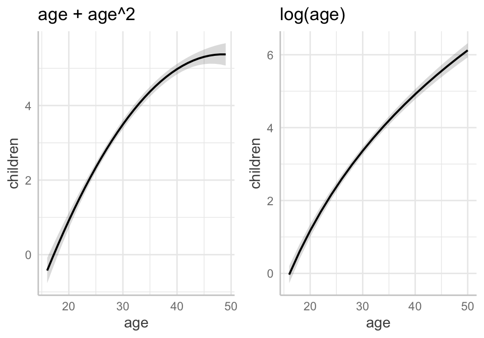
21.6.2 2. Replace the quadratic functional form of \(age\) for a logarithmic form instead, that is, replace \(age\) and its square with just \(log(age)\). What do you conclude?
mod2 <- lm(children ~ educ + log(age) + electric + heduc + radio + tv, data = fertil2)
stargazer(mod1, mod2,
          no.space = TRUE,
          header = FALSE,
          align = TRUE,
type = "html")| Dependent variable: | ||
| children | ||
| (1) | (2) | |
| educ | -0.062*** | -0.064*** |
| (0.013) | (0.013) | |
| age | 0.533*** | |
| (0.040) | ||
| I(age2) | -0.005*** | |
| (0.001) | ||
| log(age) | 5.402*** | |
| (0.167) | ||
| electric | -0.245* | -0.233* |
| (0.138) | (0.139) | |
| heduc | -0.045*** | -0.043*** |
| (0.011) | (0.011) | |
| radio | 0.146 | 0.171* |
| (0.091) | (0.092) | |
| tv | -0.385** | -0.361** |
| (0.161) | (0.162) | |
| Constant | -7.107*** | -14.599*** |
| (0.653) | (0.587) | |
| Observations | 1,953 | 1,953 |
| R2 | 0.430 | 0.422 |
| Adjusted R2 | 0.428 | 0.420 |
| Residual Std. Error | 1.734 (df = 1945) | 1.747 (df = 1946) |
| F Statistic | 209.761*** (df = 7; 1945) | 236.517*** (df = 6; 1946) |
| Note: | p<0.1; p<0.05; p<0.01 | |
Note, \(\beta_2\), or 5.402 is the predicted increase in \(\hat{children}\) for a one-unit increase in \(log(age)\), ceteris paribus. To facilitate interpretation (following the approximations in Wooldridge p.44), we can divide \(\beta_2\) by 100 to find out how much \(\hat{children}\) increases (in its own units) for a 1% increase in \(age\).
\[\begin{aligned} \Delta \hat{children} &\approx (\beta_2 /100)(\text{%} \Delta{age}) \\ \Delta \hat{children} &\approx (5.40185 /100)(\text{%} \Delta{age} ) \\ \Delta \hat{children} &\approx 0.054(\text{%} \Delta{age}) \\ \end{aligned}\]
Therefore, for every 1% increase in a woman’s age, the model predicts an increase of 0.054 children on average, holding all other factors constant.
The model with the logarithmic term does not fit the model as well as the model with the quadratic term (adjusted R^2 = 0.420 versus 0.428, respectively; SER = 1.734 versus 1.747). On that basis, one might pick Model 1 over Model 2.
21.6.3 3. Test the regression model for heteroskedasticity by using the three steps presented above and comparing it with the function provided in R for the Breusch-Pagan test.
The B-P test consists of a regression of the squared residuals on the constituent terms and then evaluating the resulting F-test for the overall significance of that regression.
21.6.3.1 Manual procedure
We’ll start by running the test models for both Model 1 (quadratic) and Model 2 (logarithmic).
# Mod 1 (quad)
dat$m1_resid <- resid(mod1)
dat$m1_residsq <- dat$m1_resid ^2
bptest_m1 <- lm(m1_residsq ~ educ + age + I(age^2) + electric + heduc + radio + tv, data = dat)
# Mod 2 (log)
dat$m2_resid <- resid(mod2)
dat$m2_resid2sq <- dat$m2_resid ^2
bptest_m2 <- lm(m2_resid2sq ~ educ + log(age) + electric + heduc + radio + tv, data = dat)
stargazer(bptest_m1, bptest_m2,
          header = FALSE,
          no.space = FALSE,
          align = TRUE,
type = "html")| Dependent variable: | ||
| m1_residsq | m2_resid2sq | |
| (1) | (2) | |
| educ | -0.165*** | -0.149*** |
| (0.036) | (0.037) | |
| age | -0.108 | |
| (0.109) | ||
| I(age2) | 0.005*** | |
| (0.002) | ||
| log(age) | 7.148*** | |
| (0.462) | ||
| electric | 0.246 | 0.295 |
| (0.373) | (0.384) | |
| heduc | -0.055* | -0.069** |
| (0.030) | (0.031) | |
| radio | 0.244 | 0.074 |
| (0.247) | (0.255) | |
| tv | -0.305 | -0.426 |
| (0.435) | (0.448) | |
| Constant | 2.001 | -20.470*** |
| (1.768) | (1.627) | |
| Observations | 1,953 | 1,953 |
| R2 | 0.168 | 0.159 |
| Adjusted R2 | 0.165 | 0.156 |
| Residual Std. Error | 4.695 (df = 1945) | 4.840 (df = 1946) |
| F Statistic | 56.159*** (df = 7; 1945) | 61.091*** (df = 6; 1946) |
| Note: | p<0.1; p<0.05; p<0.01 | |
Because we automatically get the F-statistic and its associated p-value with our model outputs, we see that we get a positive test result for both our quadratic and logarithmic form models.
For thoroughness, we can calculate F-statistics manually and then calculate their p-values.
Calculate the F statistic for the BP Test on Model 1:
\[\begin{aligned} F &= \frac{ R^2_{\hat{u}^2} / k }{ (1 - R^2_{\hat{u}^2}) / (n - k - 1) } \\ F &= \frac{ (0.1681318 / 7) } { ((1-0.1681318) / (1953-7-1)) } \\ F &= 56.1587 \\ \end{aligned}\]
## [1] 56.1587
pf(56.1587, 7, 1945, lower.tail = FALSE)## [1] 1.873915e-73Calculate the F statistic for the BP Test on Model 2:
\[\begin{aligned} F &= \frac{ R^2_{\hat{u}^2} / k }{ (1 - R^2_{\hat{u}^2}) / (n - k - 1) } \\ F &= \frac{ (0.1585037 / 6) } { ((1-0.1585037) / (1953-6-1)) } \\ F &= 61.09122 \\ \end{aligned}\]
## [1] 61.09122
pf(61.09122, 6, 1946, lower.tail = FALSE)## [1] 1.435968e-6921.6.3.2 Calculating the LM statistic
To calculate the LM statistic, we’ll use the formula provided:
\[\begin{aligned} LM &= n \times R^2_{\hat{u}^2} \\ LM &= 1953 \times 0.1681318 \\ LM &= 328.3614 \end{aligned}\]
1953 * (summary(bptest_m1)$r.squared)## [1] 328.3615
pchisq(328.3615, 7, lower.tail = FALSE)## [1] 5.254828e-67The manual B-P test (i.e. a regression of the squared residuals on the constituent terms) on Model 1 (quadratic) returns a result that is significant at the 0.001 level. This is confirmed by using lmtest::bptest().
##
##  studentized Breusch-Pagan test
##
## data:  mod1
## BP = 328.36, df = 7, p-value < 2.2e-16
Calculate the LM statistic for Model 2:
\[\begin{aligned} LM &= n \times R^2_{\hat{u}^2} \\ LM &= 1953 \times 0.1585037 \\ LM &= 309.5577 \end{aligned}\]
1953 * (summary(bptest_m2)$r.squared)## [1] 309.5577
pchisq(309.5577, 6, lower.tail = FALSE)## [1] 7.318202e-6421.7 Dealing with heteroskedasticity: Calculating robust SEs
The sandwich and lmtest packages facilitate the calculation of heteroskedastic-corrected SEs and then using them to re-test our coefficients.
First, we use sandwich::vcovHC() to extract a model’s variance-covariance matrix and adjust it to account for heteroskedasticity.
To test our coefficients, we can use lmtest::coeftest() and specify our adjusted variance-covariance matrix.
##
## t test of coefficients:
##
##                Estimate  Std. Error  t value  Pr(>|t|)
## (Intercept) -7.10706877  0.62615271 -11.3504 < 2.2e-16 ***
## educ        -0.06249197  0.01242771  -5.0284 5.399e-07 ***
## age          0.53265607  0.04183773  12.7315 < 2.2e-16 ***
## I(age^2)    -0.00549125  0.00066975  -8.1989 4.352e-16 ***
## electric    -0.24534346  0.13398537  -1.8311  0.067235 .
## heduc       -0.04495317  0.01053909  -4.2654 2.091e-05 ***
## radio        0.14573015  0.09499743   1.5340  0.125182
## tv          -0.38496679  0.14793897  -2.6022  0.009333 **
## ---
## Signif. codes:  0 '***' 0.001 '**' 0.01 '*' 0.05 '.' 0.1 ' ' 1
coeftest(mod2, vcov = mod2.hcvcov) ##
## t test of coefficients:
##
## Estimate Std. Error t value Pr(>|t|)
## (Intercept) -14.599084 0.580554 -25.1468 < 2.2e-16 ***
## educ -0.064415 0.012578 -5.1214 3.332e-07 ***
## log(age) 5.401854 0.174558 30.9459 < 2.2e-16 ***
## electric -0.233198 0.135629 -1.7194 0.08570 .
## heduc -0.043244 0.010679 -4.0492 5.340e-05 ***
## radio 0.170769 0.095975 1.7793 0.07534 .
## tv -0.360619 0.149204 -2.4170 0.01574 *
## ---
## Signif. codes: 0 '***' 0.001 '**' 0.01 '*' 0.05 '.' 0.1 ' ' 1
21.7.0.1 Using robust SEs in a stargazer table
Instead of using the coeftest() function, it’s usually more practical to replace the unadjusted SEs with robust SEs in a model reporting function.
To do this, we first have to calculate our heteroskedastic-robust SEs by taking the square-root of the diagonal of the adjusted variance-covariance matrix.
These vectors can be used in place of the standard SEs in a stargazer table using the se = list() argument.
stargazer(mod1, mod1, mod2, mod2,
          se = list(NULL, mod1.robustse, NULL, mod2.robustse),
          column.labels = c("M1 Default","M1 Robust", "M2 Default","M2 Robust"),
          no.space = FALSE,
          align = TRUE,
          header = FALSE,
          title = "Comparing normal vs robust SEs in Model 1 and Model 2",
type = "html")| Dependent variable: | ||||
| children | ||||
| M1 Default | M1 Robust | M2 Default | M2 Robust | |
| (1) | (2) | (3) | (4) | |
| educ | -0.062*** | -0.062*** | -0.064*** | -0.064*** |
| (0.013) | (0.012) | (0.013) | (0.013) | |
| age | 0.533*** | 0.533*** | ||
| (0.040) | (0.042) | |||
| I(age2) | -0.005*** | -0.005*** | ||
| (0.001) | (0.001) | |||
| log(age) | 5.402*** | 5.402*** | ||
| (0.167) | (0.175) | |||
| electric | -0.245* | -0.245* | -0.233* | -0.233* |
| (0.138) | (0.134) | (0.139) | (0.136) | |
| heduc | -0.045*** | -0.045*** | -0.043*** | -0.043*** |
| (0.011) | (0.011) | (0.011) | (0.011) | |
| radio | 0.146 | 0.146 | 0.171* | 0.171* |
| (0.091) | (0.095) | (0.092) | (0.096) | |
| tv | -0.385** | -0.385*** | -0.361** | -0.361** |
| (0.161) | (0.148) | (0.162) | (0.149) | |
| Constant | -7.107*** | -7.107*** | -14.599*** | -14.599*** |
| (0.653) | (0.626) | (0.587) | (0.581) | |
| Observations | 1,953 | 1,953 | 1,953 | 1,953 |
| R2 | 0.430 | 0.430 | 0.422 | 0.422 |
| Adjusted R2 | 0.428 | 0.428 | 0.420 | 0.420 |
| Residual Std. Error | 1.734 (df = 1945) | 1.734 (df = 1945) | 1.747 (df = 1946) | 1.747 (df = 1946) |
| F Statistic | 209.761*** (df = 7; 1945) | 209.761*** (df = 7; 1945) | 236.517*** (df = 6; 1946) | 236.517*** (df = 6; 1946) |
| Note: | p<0.1; p<0.05; p<0.01 | |||