1 Week 1: A Primer on Using Text as Data
1.1 Setup
For this first example, we will replicate (and extend) Mendenhall’s (1887) and Mendenhall’s (1901) studies of word-length distribution.
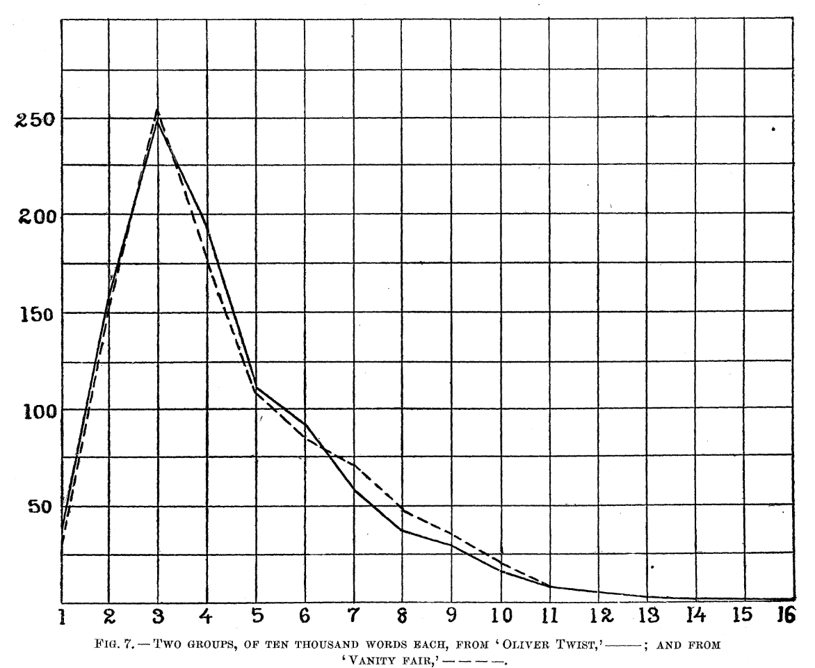
Figure 1.1: From Mendenhall (1987) - The Characteristic Curves of Composition.
First we load the packages that we’ll be using:
library(tidyverse) # for wrangling data
library(tidylog) # to know what we are wrangling
library(tidytext) # for 'tidy' manipulation of text data
library(wesanderson) # to prettify
library(gutenbergr) # to get some books
library(kableExtra) # for displaying data in html format (relevant for formatting this worksheet mainly)
1.2 Get Data
Mendenhall (1887) argued that “every writer makes use of a vocabulary which is peculiar to himself, and the character of which does not materially change from year to year during his productive [years],” and that one of these characteristics was word length. Mendenhall (1901) takes this further and suggests that, given this assumption, Shakespeare and Bacon were not the same person1.
Let’s get a corpus–a collection of documents–that we can analyze. We can search the Gutenberg repository and create a corpus with selected works.
# Inspect Project Gutenberg metadata to find all texts authored by Oscar Wilde.
# This returns a table of matching Gutenberg entries (including IDs you can use to download texts).
gutenberg_metadata %>%
  filter(author == "Wilde, Oscar")
## # A tibble: 67 × 8
## gutenberg_id title author
## <int> <chr> <chr>
## 1 174 The Picture of Dorian… Wilde…
## 2 301 The Ballad of Reading… Wilde…
## 3 773 Lord Arthur Savile's … Wilde…
## 4 774 Essays and Lectures Wilde…
## 5 790 Lady Windermere's Fan Wilde…
## 6 844 The Importance of Bei… Wilde…
## 7 854 A Woman of No Importa… Wilde…
## 8 873 A House of Pomegranat… Wilde…
## 9 875 The Duchess of Padua Wilde…
## 10 885 An Ideal Husband Wilde…
## # ℹ 57 more rows
## # ℹ 5 more variables:
## # gutenberg_author_id <int>,
## # language <fct>,
## # gutenberg_bookshelf <chr>, rights <fct>,
## # has_text <lgl>1.3 Word Length in Wilde’s Corpus
That’s a lot of Wilde! Let’s focus on four plays: “The Importance of Being Earnest”, “A Woman of No Importance”, “Lady Windermere’s Fan”, and “An Ideal Husband”. We can download all of these plays using their Gutenberg ID numbers:
# Download four Oscar Wilde plays from Project Gutenberg using their Gutenberg IDs.
# The IDs correspond to specific texts in the Gutenberg catalog.
# `meta_fields` appends the requested metadata (here: title and author) to each row of text.
wilde <- gutenberg_download(
  c(790, 844, 854, 885),
  meta_fields = c("title", "author")
)

# Quick inspection: print rows 51–75 (often useful for seeing the structure of the raw text)
# and show up to 25 rows in the console output.
print(n = 25, wilde[c(51:75), ])
## # A tibble: 25 × 4
## gutenberg_id text title author
## <int> <chr> <chr> <chr>
## 1 790 "" Lady… Wilde…
## 2 790 "" Lady… Wilde…
## 3 790 "THE PERSONS OF… Lady… Wilde…
## 4 790 "" Lady… Wilde…
## 5 790 "" Lady… Wilde…
## 6 790 "Lord Windermer… Lady… Wilde…
## 7 790 "" Lady… Wilde…
## 8 790 "Lord Darlingto… Lady… Wilde…
## 9 790 "" Lady… Wilde…
## 10 790 "Lord Augustus … Lady… Wilde…
## 11 790 "" Lady… Wilde…
## 12 790 "Mr. Dumby" Lady… Wilde…
## 13 790 "" Lady… Wilde…
## 14 790 "Mr. Cecil Grah… Lady… Wilde…
## 15 790 "" Lady… Wilde…
## 16 790 "Mr. Hopper" Lady… Wilde…
## 17 790 "" Lady… Wilde…
## 18 790 "Parker, Butler" Lady… Wilde…
## 19 790 "" Lady… Wilde…
## 20 790 " … Lady… Wilde…
## 21 790 "" Lady… Wilde…
## 22 790 "Lady Windermer… Lady… Wilde…
## 23 790 "" Lady… Wilde…
## 24 790 "The Duchess of… Lady… Wilde…
## 25 790 "" Lady… Wilde…In this case, the unit of analysis is something like a line. We are interested in each word–also known as a token–and its length within each play. We will clean some unwanted text–text that would only add noise to our analysis–and then count the number of words.
wilde <- wilde %>%
  # Standardize the title for "The Importance of Being Earnest"
  # (Gutenberg titles can vary slightly across editions/records).
  mutate(
    title = ifelse(
      str_detect(title, "Importance of Being"),
      "The Importance of Being Earnest",
      title
    )
  ) %>%
  # Remove empty lines (blank rows add noise and can affect tokenization/counts).
  filter(text != "") %>%
  # Remove speaker labels typical of plays (often written in ALL CAPS).
  # This keeps primarily spoken text rather than character-name headers.
  filter(str_detect(text, "[A-Z]{3,}") == FALSE)
## mutate: changed 3,884 values (27%) of 'title' (0 new NAs)
## filter: removed 4,232 rows (29%), 10,303 rows remaining
## filter: removed 4,207 rows (41%), 6,096 rows remaining
# Inspect a slice of the cleaned text to confirm the filters behaved as expected.
print(n = 25, wilde[c(51:75), ])
## # A tibble: 25 × 4
## gutenberg_id text title author
## <int> <chr> <chr> <chr>
## 1 790 "tea-table L._ … Lady… Wilde…
## 2 790 "home to any on… Lady… Wilde…
## 3 790 " … Lady… Wilde…
## 4 790 "he’s come." Lady… Wilde…
## 5 790 "hands with you… Lady… Wilde…
## 6 790 "lovely? They … Lady… Wilde…
## 7 790 "table_.] And … Lady… Wilde…
## 8 790 "everything. I… Lady… Wilde…
## 9 790 "present to me.… Lady… Wilde…
## 10 790 "life, isn’t it… Lady… Wilde…
## 11 790 "down. [_Still… Lady… Wilde…
## 12 790 "birthday, Lady… Lady… Wilde…
## 13 790 "front of your … Lady… Wilde…
## 14 790 "you." Lady… Wilde…
## 15 790 " … Lady… Wilde…
## 16 790 "Foreign Office… Lady… Wilde…
## 17 790 "with her pocke… Lady… Wilde…
## 18 790 "Won’t you come… Lady… Wilde…
## 19 790 "miserable, Lad… Lady… Wilde…
## 20 790 "table L._]" Lady… Wilde…
## 21 790 "whole evening." Lady… Wilde…
## 22 790 "that the only … Lady… Wilde…
## 23 790 "things we _can… Lady… Wilde…
## 24 790 "You mustn’t la… Lady… Wilde…
## 25 790 "don’t see why … Lady… Wilde…Now, we can change our unit of analysis to the token:
wilde_words <- wilde %>%
  # Tokenize: split the `text` column into one word per row.
  # The output column is named `word`; punctuation is removed and words are lowercased by default.
  unnest_tokens(word, text) %>%
  # Remove underscores (some Gutenberg texts include formatting artifacts like "_" that add noise).
  mutate(word = str_remove_all(word, "\\_"))
## mutate: changed 1,225 values (2%) of 'word'
## (0 new NAs)
# View the tokenized dataset (one row per token, with title/author carried along).
wilde_words
## # A tibble: 60,477 × 4
## gutenberg_id title author word
## <int> <chr> <chr> <chr>
## 1 790 Lady Windermere… Wilde… by
## 2 790 Lady Windermere… Wilde… sixt…
## 3 790 Lady Windermere… Wilde… edit…
## 4 790 Lady Windermere… Wilde… first
## 5 790 Lady Windermere… Wilde… publ…
## 6 790 Lady Windermere… Wilde… 1893
## 7 790 Lady Windermere… Wilde… first
## 8 790 Lady Windermere… Wilde… issu…
## 9 790 Lady Windermere… Wilde… by
## 10 790 Lady Windermere… Wilde… meth…
## # ℹ 60,467 more rowsThat’s a lot of words! We will now create a column for word length, and then count the number of words by length (by play!).
wilde_words_ct <- wilde_words %>%
  # Compute the length (number of characters) of each token
  mutate(word_length = str_length(word)) %>%
  # Group by play title and word length to build the word-length distribution
  group_by(word_length, title) %>%
  # Count how many tokens fall into each (word_length, title) bin
  # (n() returns the group size; mutate repeats it on every row in the group)
  mutate(total_word_length = n()) %>%
  # Keep a single row per (word_length, title) combination
  distinct(word_length, title, .keep_all = TRUE) %>%
  # Keep only the variables needed for plotting/inspection
  dplyr::select(word_length, title, author, total_word_length)
## mutate: new variable 'word_length' (integer) with 17 unique values and 0% NA
## group_by: 2 grouping variables (word_length, title)
## mutate (grouped): new variable 'total_word_length' (integer) with 58 unique values and 0% NA
## distinct (grouped): removed 60,415 rows (>99%), 62 rows remaining (removed 0 groups, 62 groups remaining)Let’s see the distribution of word length by play:
wilde_words_ct %>%
  # Plot the word-length distribution for each play
  ggplot(aes(x = word_length, y = total_word_length, color = title)) +
  # Points show observed counts at each word length
  geom_point(alpha = 0.8) +
  # Lines connect points to make the distribution shape easier to see
  geom_line(alpha = 0.8) +
  # Use a Wes Anderson palette for play colors
  scale_color_manual(values = wes_palette("Royal2")) +
  # Clean, minimal theme
  theme_minimal() +
  # Place legend on the right for readability
  theme(legend.position = "right") +
  # Axis labels (x = word length in characters; y = number of tokens of that length)
  labs(x = "Length", y = "Total Number of Words", color = "")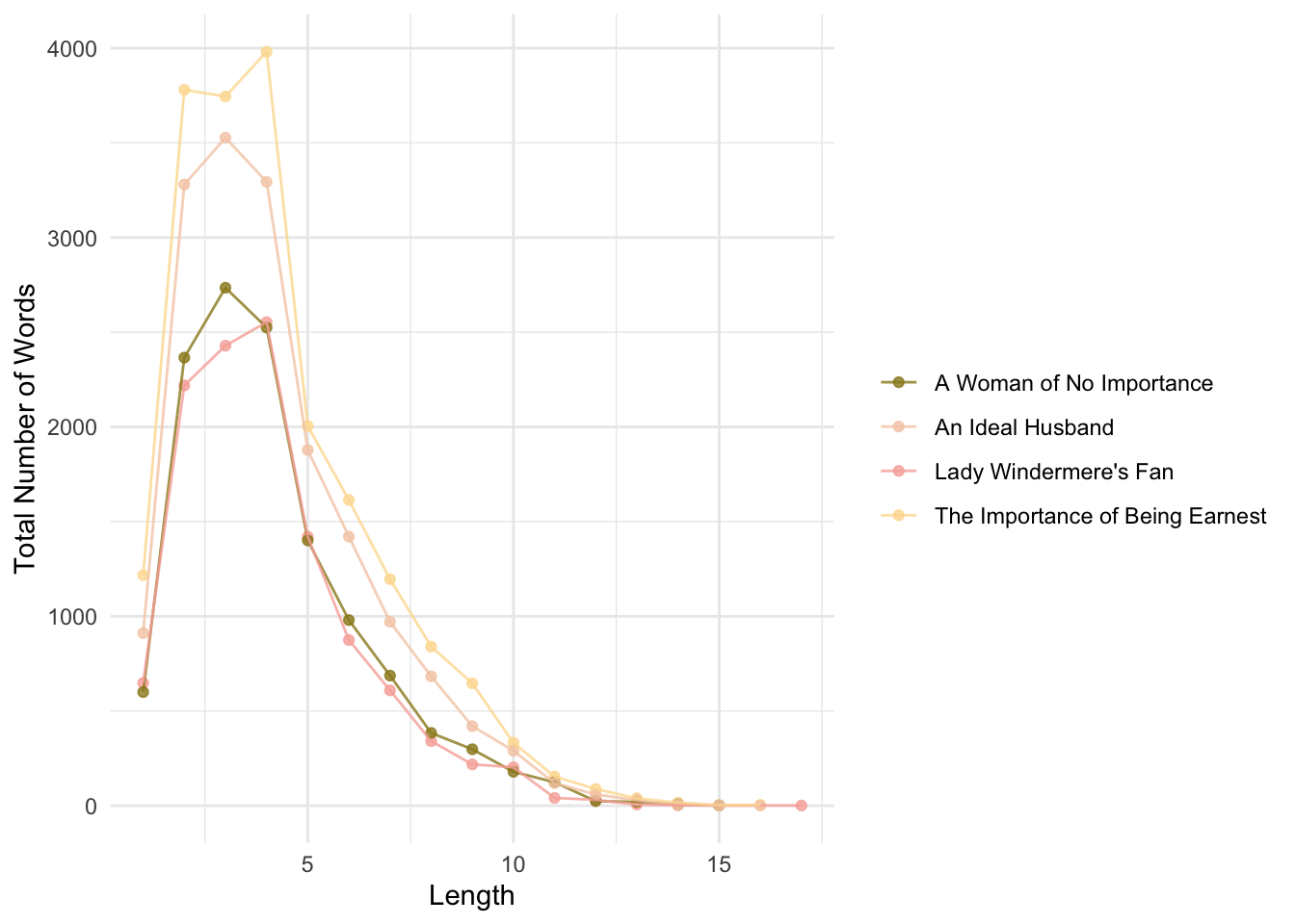
This is a problem. Why?
Here is a solution (proposed by Mendenhall):
wilde_words %>%
  # Work within each play separately
  group_by(title) %>%
  # Take an equal-sized random sample of tokens from each play
  # (this makes the resulting distributions comparable across plays)
  slice_sample(n = 10000) %>%
  # Compute word length for each token, and the median word length within each play (on the sampled data)
  mutate(
    word_length = str_length(word),
    median_word_length = median(word_length)
  ) %>%
  # Count how many sampled tokens fall into each word-length bin, within each play
  group_by(word_length, title) %>%
  mutate(total_word_length = n()) %>%
  # Keep one row per (word_length, title) combination for plotting
  distinct(word_length, title, .keep_all = TRUE) %>%
  # Keep relevant columns (median_word_length is repeated but useful for plotting the median line)
  dplyr::select(word_length, title, author, total_word_length, median_word_length) %>%
  # Plot the sampled word-length distributions
  ggplot(aes(x = word_length, y = total_word_length, color = title)) +
  geom_point(alpha = 0.8) +
  geom_line(alpha = 0.8) +
  # Add a vertical line at each play's median word length
  geom_vline(aes(xintercept = median_word_length, color = title, linetype = title)) +
  scale_color_manual(values = wes_palette("Royal2")) +
  theme_minimal() +
  theme(legend.position = "right") +
  labs(
    x = "Length",
    y = "Total Number of Words",
    color = "",
    linetype = "",
    caption = "Note: Line type shows median word length."
  )
## group_by: one grouping variable (title)
## slice_sample (grouped): removed 20,477 rows (34%), 40,000 rows remaining (removed 0 groups, 4 groups remaining)
## mutate (grouped): new variable 'word_length' (integer) with 17 unique values and 0% NA
## new variable 'median_word_length' (double) with one unique value and 0% NA
## group_by: 2 grouping variables (word_length, title)
## mutate (grouped): new variable 'total_word_length' (integer) with 57 unique values and 0% NA
## distinct (grouped): removed 39,939 rows (>99%), 61 rows remaining (removed 0 groups, 61 groups remaining)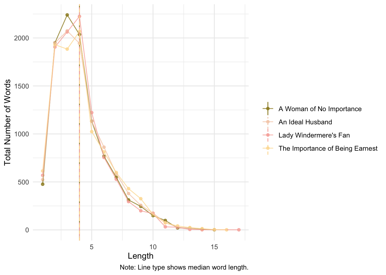
Would you look at that, Mendenhall was onto something: an author may have a signature in terms of word-length distribution. For Wilde, there is no obvious change across time (each play was published in a different year). But what happens when we compare Wilde’s signature with Shakespeare’s? Let’s choose four plays (at random) by Shakespeare: A Midsummer Night’s Dream, The Merchant of Venice, Much Ado About Nothing, and The Tempest.
1.4 Comparing Shakespeare and Wilde
shakes <- gutenberg_download(c(1520,2242,2243,2235),
                             meta_fields = c("title","author"))
print(n=25,shakes[c(51:75),])
## # A tibble: 25 × 4
## gutenberg_id text title author
## <int> <chr> <chr> <chr>
## 1 1520 "[Enter Leonato… Much… Shake…
## 2 1520 "" Much… Shake…
## 3 1520 "Leon." Much… Shake…
## 4 1520 "I learn in thi… Much… Shake…
## 5 1520 "night to Messi… Much… Shake…
## 6 1520 "" Much… Shake…
## 7 1520 "Mess." Much… Shake…
## 8 1520 "He is very nea… Much… Shake…
## 9 1520 "left him." Much… Shake…
## 10 1520 "" Much… Shake…
## 11 1520 "Leon." Much… Shake…
## 12 1520 "How many gentl… Much… Shake…
## 13 1520 "" Much… Shake…
## 14 1520 "Mess." Much… Shake…
## 15 1520 "But few of any… Much… Shake…
## 16 1520 "" Much… Shake…
## 17 1520 "Leon." Much… Shake…
## 18 1520 "A victory is t… Much… Shake…
## 19 1520 "numbers. I fi… Much… Shake…
## 20 1520 "a young Floren… Much… Shake…
## 21 1520 "" Much… Shake…
## 22 1520 "Mess." Much… Shake…
## 23 1520 "Much deserved … Much… Shake…
## 24 1520 "He hath borne … Much… Shake…
## 25 1520 "in the figure … Much… Shake…This text is cleaner than Wilde’s corpus, so we will leave it as is. Also, it is harder to systematically remove the name of the person speaking. Is this a problem? Why? Why not?
We can put together both corpora and see differences in the distributions of word length.
shakes_words <- shakes %>%
  # Filter out all empty rows
  filter(text != "") %>%
  # This is a play. The name of each character before they speak
  filter(str_detect(text,"[A-Z]{3,}")==FALSE) %>%
  # take the column text and divide it by words
  unnest_tokens(word, text)
## filter: removed 2,582 rows (23%), 8,821 rows remaining
## filter: removed 28 rows (<1%), 8,793 rows remaining
# Bind both word dfs
words <- rbind.data.frame(shakes_words,wilde_words)

# Count words etc.
words %>%
  group_by(title,author) %>%
  slice_sample(n=10000) %>%
  mutate(word_length = str_length(word),
         median_word_length = median(word_length)) %>%
  group_by(word_length,title,author) %>%
  mutate(total_word_length = n()) %>%
  distinct(word_length,title,.keep_all=T) %>%
  dplyr::select(word_length,title,author,total_word_length,median_word_length) %>%
  ggplot(aes(y=total_word_length,x=word_length,color=author,group=title)) +
  geom_point(alpha=0.8) +
  geom_line(alpha=0.8) +
  scale_color_manual(values = wes_palette("Royal2")) +
  # facet_wrap(~author, ncol = 2)+
  theme_minimal() +
  theme(legend.position = "bottom") +
  labs(x="Length", y = "Total Number of Words", color = "", linetype = "",
       caption = "Note: Median word length is 4 for both authors.")
## group_by: 2 grouping variables (title, author)
## slice_sample (grouped): removed 53,665 rows (43%), 70,000 rows remaining (removed 0 groups, 7 groups remaining)
## mutate (grouped): new variable 'word_length' (integer) with 17 unique values and 0% NA
## new variable 'median_word_length' (double) with one unique value and 0% NA
## group_by: 3 grouping variables (word_length, title, author)
## mutate (grouped): new variable 'total_word_length' (integer) with 88 unique values and 0% NA
## distinct (grouped): removed 69,894 rows (>99%), 106 rows remaining (removed 0 groups, 106 groups remaining)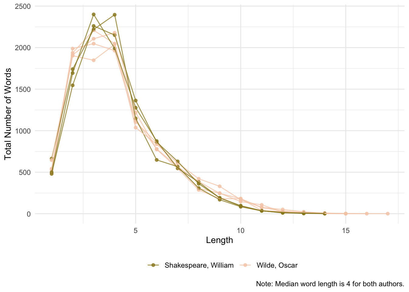
Are there any differences? What can we conclude from the evidence? What are the limitations of this approach? Are there alternative approaches to study what Mendenhall was getting at?
1.5 Exercise (Optional)
- Extend the current analysis to other authors or to more works by the same author.
- Are there better ways to compare the distribution of word length? Are there changes across time? Are there differences between different types of works (e.g., fiction vs. non-fiction, prose vs. poetry)?
1.6 Final Words
As will often be the case, we won’t be able to cover every single feature that the different packages have to offer, show every object we create, or explore everything we can do with them. My advice is that you go home and explore the code in detail. Try applying it to a different corpus and come to the next class with questions (or just show off what you were able to do).