2 Week 2: Tokenization and Word Frequency
Slides
- 3 Tokenization and Word Frequency (link or in Perusall)
2.1 Setup
As always, we first load the packages that we’ll be using:
library(tidyverse) # for wrangling data
library(tidylog) # to know what we are wrangling
library(tidytext) # for 'tidy' manipulation of text data
library(quanteda) # tokenization power house
library(quanteda.textstats)
library(quanteda.textplots)
library(wesanderson) # to prettify
library(readxl) # to read excel
library(kableExtra) # for displaying data in html format (relevant for formatting this worksheet mainly)
2.2 Get Data:
For this example, we will be using small corpus of song lyrics.
sample_lyrics <- read_excel("data/lyrics_sample.xlsx")
head(sample_lyrics)
## # A tibble: 6 × 5
## artist album year song lyrics
## <chr> <chr> <dbl> <chr> <chr>
## 1 Rage Against the … Evil… 1996 Bull… "Come…
## 2 Rage Against the … Rage… 1992 Kill… "Kill…
## 3 Rage Against the … Rene… 2000 Rene… "No m…
## 4 Rage Against the … The … 1999 Slee… "Yeah…
## 5 Rage Against the … The … 1999 Guer… "Tran…
## 6 Rage Against the … The … 1999 Test… "Uh!\…Ok, so we have different artists, from different genres and years…
##
##      Megan Thee Stallion
##                        5
## Rage Against the Machine
##                        6
##         System of a Down
##                        5
##             Taylor Swift
##                        5
And we have the lyrics in the following form:
## [1] "Yeah\r\n\r\nThe world is my expense\r\nIt’s the cost of my desire\r\nJesus blessed me with its future\r\nAnd I protect it with fire\r\n\r\nSo raise your fists and march around\r\nJust don’t take what you need\r\nI’ll jail and bury those committed\r\nAnd smother the rest in greed\r\n\r\nCrawl with me into tomorrow\r\nOr I’ll drag you to your grave\r\nI’m deep inside your children\r\nThey’ll betray you in my name\r\n\r\nHey, hey, sleep now in the fire\r\nHey, hey, sleep now in the fire\r\n\r\nThe lie is my expense\r\nThe scope of my desire\r\nThe party blessed me with its future\r\nAnd I protect it with fire\r\n\r\nI am the Niña, the Pinta, the Santa María\r\nThe noose and the rapist, the fields overseer\r\nThe Agents of Orange, the Priests of Hiroshima\r\nThe cost of my desire, sleep now in the fire\r\n\r\nHey, hey, sleep now in the fire\r\nHey, hey, sleep now in the fire\r\n\r\nFor it’s the end of history\r\nIt’s caged and frozen still\r\nThere is no other pill to take\r\nSo swallow the one that made you ill\r\n\r\nThe Niña, the Pinta, the Santa María\r\nThe noose and the rapist, the fields overseer\r\nThe Agents of Orange, the Priests of Hiroshima\r\nThe cost of my desire to sleep now in the fire\r\n\r\nYeah\r\n\r\nSleep now in the fire\r\nSleep now in the fire\r\nSleep now in the fire\r\nSleep now in the fire"2.3 Cleaning the Text
Much like music, text comes in different forms and qualities. From the Regex workshop, you might remember that special characters can signal, for example, a new line (\n) or a carriage return (\r). For this example, we can remove them2. Before working with text, always check the state of your documents once they are loaded into your program of choice.
sample_lyrics <- sample_lyrics %>%
  # Replace newline characters (\n) with a period.
  # Note: "\\n" matches the literal newline escape sequence in the string.
  mutate(
    lyrics_clean = str_replace_all(lyrics, "\\n", "\\."),
    # Replace carriage returns (\r) with a period as well.
    lyrics_clean = str_replace_all(lyrics_clean, "\\r", "\\.")
  ) %>%
  # Drop the original lyrics column to avoid keeping both raw and cleaned versions
  dplyr::select(-lyrics)
## mutate: new variable 'lyrics_clean'
## (character) with 21 unique values and 0% NA
# Inspect the 4th cleaned lyric to confirm the replacements worked as intended
sample_lyrics$lyrics_clean[4]
## [1] "Yeah....The world is my expense..It’s the cost of my desire..Jesus blessed me with its future..And I protect it with fire....So raise your fists and march around..Just don’t take what you need..I’ll jail and bury those committed..And smother the rest in greed....Crawl with me into tomorrow..Or I’ll drag you to your grave..I’m deep inside your children..They’ll betray you in my name....Hey, hey, sleep now in the fire..Hey, hey, sleep now in the fire....The lie is my expense..The scope of my desire..The party blessed me with its future..And I protect it with fire....I am the Niña, the Pinta, the Santa María..The noose and the rapist, the fields overseer..The Agents of Orange, the Priests of Hiroshima..The cost of my desire, sleep now in the fire....Hey, hey, sleep now in the fire..Hey, hey, sleep now in the fire....For it’s the end of history..It’s caged and frozen still..There is no other pill to take..So swallow the one that made you ill....The Niña, the Pinta, the Santa María..The noose and the rapist, the fields overseer..The Agents of Orange, the Priests of Hiroshima..The cost of my desire to sleep now in the fire....Yeah....Sleep now in the fire..Sleep now in the fire..Sleep now in the fire..Sleep now in the fire"2.4 Tokenization
Our goal is to create a document-feature matrix, from which we will later extract information about word frequency. To do that, we start by creating a corpus object using the quanteda package.
# Create a quanteda corpus from the cleaned lyrics data frame.
# - text_field specifies which column contains the text to be treated as documents.
# - unique_docnames ensures each document gets a unique ID (useful when rows might share names/IDs).
corpus_lyrics <- corpus(
  sample_lyrics,
  text_field = "lyrics_clean",
  unique_docnames = TRUE
)

# Quick overview of the corpus (number of documents, tokens, etc.)
summary(corpus_lyrics)
## Corpus consisting of 21 documents, showing 21 documents:
##
## Text Types Tokens Sentences
## text1 119 375 35
## text2 52 853 83
## text3 188 835 91
## text4 97 352 38
## text5 160 440 50
## text6 133 535 67
## text7 105 560 53
## text8 67 366 40
## text9 68 298 33
## text10 65 258 32
## text11 137 558 68
## text12 131 876 70
## text13 159 465 41
## text14 162 544 62
## text15 196 738 84
## text16 169 549 50
## text17 229 867 55
## text18 193 664 61
## text19 310 1190 87
## text20 198 656 48
## text21 255 1092 73
## artist
## Rage Against the Machine
## Rage Against the Machine
## Rage Against the Machine
## Rage Against the Machine
## Rage Against the Machine
## Rage Against the Machine
## System of a Down
## System of a Down
## System of a Down
## System of a Down
## System of a Down
## Taylor Swift
## Taylor Swift
## Taylor Swift
## Taylor Swift
## Taylor Swift
## Megan Thee Stallion
## Megan Thee Stallion
## Megan Thee Stallion
## Megan Thee Stallion
## Megan Thee Stallion
## album year
## Evil Empire 1996
## Rage Against the Machine 1992
## Renegades 2000
## The Battle of Los Angeles 1999
## The Battle of Los Angeles 1999
## The Battle of Los Angeles 1999
## Mezmerize 2005
## Toxicity 2001
## Toxicity 2001
## Toxicity 2001
## Toxicity 2001
## 1989 2014
## Midnights 2022
## Fearless 2008
## 1989 2014
## Fearless 2008
## Traumazine 2022
## Suga 2020
## Something for Thee Hotties 2021
## Traumazine 2022
## Traumazine 2022
## song
## Bulls on Parade
## Killing in the Name
## Renegades of Funk
## Sleep Now in the Fire
## Guerrilla Radio
## Testify
## B.Y.O.B
## Chop Suey!
## Aerials
## Toxicty
## Sugar
## Shake it Off
## Anti-Hero
## You Belong With Me
## Blank Space
## Love Story
## Plan B
## Savage
## Thot Shit
## Her
## UngratefulLooks good. Now we can tokenize our corpus (and reduce complexity). One benefit of creating a corpus object first is that it preserves all the metadata for each document when we tokenize. This will come in handy later.
# Tokenize the corpus: split each document into tokens (typically words).
# Here we remove some elements that usually add noise for word-frequency analysis.
lyrics_toks <- tokens(
  corpus_lyrics,
  remove_numbers = TRUE,  # remove tokens that are numbers (are these relevant?)
  remove_punct   = TRUE,  # remove punctuation marks (e.g., commas, periods)
  remove_url     = TRUE   # remove URLs (useful if lyrics contain links/metadata)
)

# Inspect a couple of tokenized documents (documents 4 and 14)
lyrics_toks[c(4, 14)]
## Tokens consisting of 2 documents and 4 docvars.
## text4 :
## [1] "Yeah" "The" "world" "is"
## [5] "my" "expense" "It’s" "the"
## [9] "cost" "of" "my" "desire"
## [ ... and 227 more ]
##
## text14 :
## [1] "You're" "on" "the"
## [4] "phone" "with" "your"
## [7] "girlfriend" "she's" "upset"
## [10] "She's" "going" "off"
## [ ... and 385 more ]We got rid of punctuation. Now let’s remove stop words, high- and low-frequency words, and stem the remaining tokens. Here I am cheating, though: I already know which words are high- and low-frequency because I inspected my dfm (see the next code chunk).
# Remove stopwords and any additional terms you want to drop before building a dfm.
# - stopwords(language = "en") provides a standard English stopword list.
# - You can add/remove terms depending on your corpus and research question.
# - padding = FALSE drops removed tokens entirely (no placeholder tokens are kept).
lyrics_toks <- tokens_remove(
  lyrics_toks,
  c(
    stopwords(language = "en"),
    # "now" is very frequent in this corpus (identified after inspecting the dfm),
    # and it is not substantively useful for our purposes here.
    "now"
  ),
  padding = FALSE
)

# Stem tokens to reduce inflected/derived words to a common root
# (e.g., "running", "runs" -> "run"), which reduces vocabulary size.
lyrics_toks_stem <- tokens_wordstem(lyrics_toks, language = "en")

# Compare the tokenized text before and after stemming for two example documents
lyrics_toks[c(4, 14)]
## Tokens consisting of 2 documents and 4 docvars.
## text4 :
## [1] "Yeah" "world" "expense" "It’s"
## [5] "cost" "desire" "Jesus" "blessed"
## [9] "future" "protect" "fire" "raise"
## [ ... and 105 more ]
##
## text14 :
## [1] "phone" "girlfriend" "upset"
## [4] "going" "something" "said"
## [7] "Cause" "get" "humor"
## [10] "like" "room" "typical"
## [ ... and 133 more ]
lyrics_toks_stem[c(4, 14)]## Tokens consisting of 2 documents and 4 docvars.
## text4 :
## [1] "Yeah" "world" "expens" "It’s"
## [5] "cost" "desir" "Jesus" "bless"
## [9] "futur" "protect" "fire" "rais"
## [ ... and 105 more ]
##
## text14 :
## [1] "phone" "girlfriend" "upset"
## [4] "go" "someth" "said"
## [7] "Caus" "get" "humor"
## [10] "like" "room" "typic"
## [ ... and 133 more ]We can compare the stemmed output and the non-stemmed output. Why did “future” become “futur”? Because stemming assumes that, for our purposes, “future” and “futuristic” should be treated as the same underlying root. Whether that assumption is appropriate depends on your research question. Finally, we can create our document-feature matrix (dfm).
# Create a document-feature matrix (dfm) from the tokens.
# Rows = documents; columns = features (typically word types); cells = feature counts.
lyrics_dfm <- dfm(lyrics_toks)

# Create a dfm from the stemmed tokens to further reduce vocabulary size.
lyrics_dfm_stem <- dfm(lyrics_toks_stem)

# Inspect the first few rows/columns of the stemmed dfm
head(lyrics_dfm_stem)
## Document-feature matrix of: 6 documents, 1,161 features (93.10% sparse) and 4 docvars.
## features
## docs come wit microphon explod shatter
## text1 4 4 1 1 1
## text2 2 0 0 0 0
## text3 0 0 0 0 0
## text4 0 0 0 0 0
## text5 0 0 0 0 0
## text6 0 4 0 0 0
## features
## docs mold either drop hit like
## text1 1 1 3 1 1
## text2 0 0 0 0 0
## text3 0 0 0 0 4
## text4 0 0 0 0 0
## text5 0 0 0 0 1
## text6 0 0 0 0 0
## [ reached max_nfeat ... 1,151 more features ]Note that once we create the dfm object, all tokens become lowercase. Now we can check what are the 15 most frequent tokens.
lyrics_dfm_stem %>%
  # Compute the top n most frequent features (tokens) in the dfm
  textstat_frequency(n = 30) %>%
  # Plot the top features as a horizontal bar chart
  ggplot(aes(
    x = reorder(feature, frequency),
    y = frequency,
    fill = frequency,
    color = frequency
  )) +
  # Use bars to show counts (alpha makes them slightly transparent)
  geom_col(alpha = 0.5) +
  # Flip coordinates so feature labels are easier to read
  coord_flip() +
  # Fix ordering after coord_flip when using reorder()
  scale_x_reordered() +
  # Map frequency to color/fill gradients for visual emphasis
  scale_color_distiller(palette = "PuOr") +
  scale_fill_distiller(palette = "PuOr") +
  # Clean theme
  theme_minimal() +
  labs(x = "", y = "Frequency", color = "", fill = "") +
  # Hide legend (frequency is already shown on the y-axis)
  theme(legend.position = "none")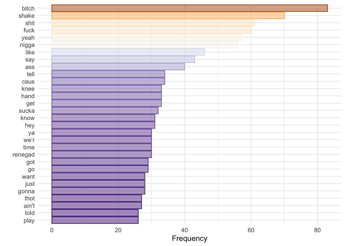
Does not tell us much, but I used the previous code to check for low-information tokens that I might want to remove from my analysis. We can also see how many tokens appear only once:
only_once <- lyrics_dfm_stem %>%
  textstat_frequency() %>%
  filter(frequency == 1)
## filter: removed 564 rows (49%), 597 rows
## remaining
length(only_once$feature)## [1] 597More interesting for text analysis is to count words over time/space. In this case, our ‘space’ can be the artist.
lyrics_dfm_stem %>%
  # Compute top features *within each artist* (grouped frequency table)
  textstat_frequency(n = 15, groups = c(artist)) %>%
  ggplot(aes(
    x = reorder_within(feature, frequency, group), # reorder features separately within each facet
    y = frequency,
    fill = group,
    color = group
  )) +
  geom_col(alpha = 0.5) +
  coord_flip() +
  # One panel per artist; free scales so each artist's frequency range can differ
  facet_wrap(~group, scales = "free") +
  # Fix axis ordering after reorder_within() + coord_flip()
  scale_x_reordered() +
  scale_color_brewer(palette = "PuOr") +
  scale_fill_brewer(palette = "PuOr") +
  theme_minimal() +
  labs(x = "", y = "", color = "", fill = "") +
  theme(legend.position = "none")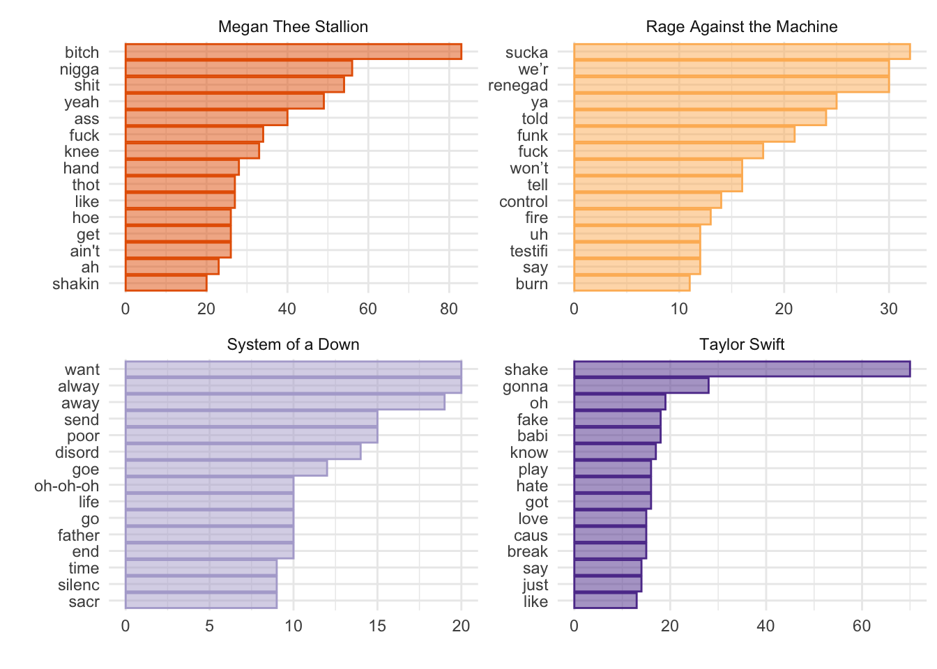
Interesting. There is not a lot of overlap (apart from one token shared by Megan Thee Stallion and Rage Against the Machine). However, it would be great if we could measure the importance of a word relative to how widely it appears across documents (i.e., normalize by document prevalence). Enter TF-IDF: “term frequency–inverse document frequency.” TF-IDF weighting up-weights relatively rare words–words that do not appear in many documents. By combining term frequency and inverse document frequency, we can identify words that are especially characteristic of a given document within a collection.
lyrics_dfm_tfidf <- dfm_tfidf(lyrics_dfm_stem) # Create a dfm with tf-idf instead of counts

lyrics_dfm_tfidf %>%
  # force = TRUE ensures features are computed within groups even if some groups have sparse features
  textstat_frequency(n = 15, groups = c(artist), force = TRUE) %>%
  ggplot(aes(x = reorder_within(feature, frequency, group), y = frequency, fill = group, color = group)) +
  geom_col(alpha = 0.5) +
  coord_flip() +
  facet_wrap(~group, scales = "free") +
  scale_x_reordered() +
  scale_color_brewer(palette = "PuOr") +
  scale_fill_brewer(palette = "PuOr") +
  theme_minimal() +
  labs(x = "", y = "TF-IDF", color = "", fill = "") +
  theme(legend.position = "none")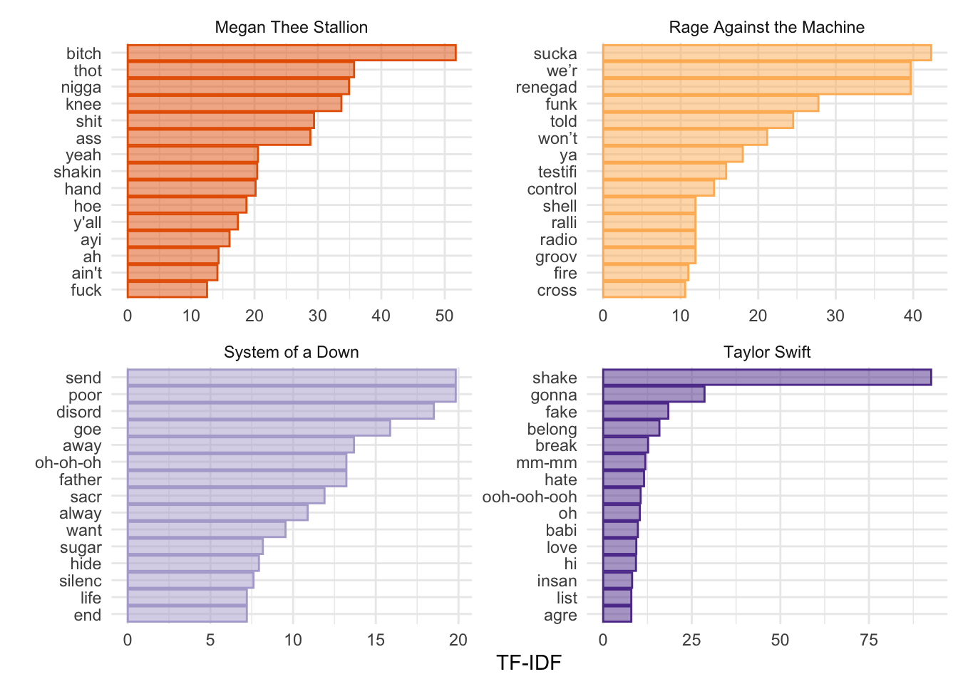
If we are building a dictionary, for example, we might want to include words with high TF-IDF values. Another way to think about TF-IDF is in terms of predictive power. Words that are common to all documents have little predictive power and receive a TF-IDF value close to 0. Words that appear in only a relatively small number of documents tend to have greater predictive power and receive higher TF-IDF values. Very rare words are also effectively down-weighted, since they may provide only idiosyncratic information about a single document (i.e., strong “prediction” for one document but little information about the rest). As you will read in Chapters 6–7 of Grimmer et al., the goal is to find the right balance.
Another useful tool (and concept) is keyness. Keyness is a two-by-two association score for features that occur differentially across categories. We can estimate which features are more strongly associated with one category (in this case, one artist) relative to another. Let’s compare Megan Thee Stallion and Taylor Swift.
# Subset the dfm to include only documents after 2006.
# This is a convenient way to focus on a time period where both artists are likely represented.
lyrics_dfm_ts_mts <- dfm_subset(lyrics_dfm_stem, year > 2006)

# Compute keyness statistics (a differential association measure) for each feature.
# - target defines the "focus" group: here, documents where artist == "Taylor Swift".
# - The resulting object ranks features by how strongly they are associated with the target group
#   versus the reference group (all other documents in the dfm, here: non–Taylor Swift).
lyrics_key <- textstat_keyness(
  lyrics_dfm_ts_mts,
  target = lyrics_dfm_ts_mts$artist == "Taylor Swift"
)

# Visualize the most strongly associated (key) features for the target vs. the reference group.
textplot_keyness(lyrics_key)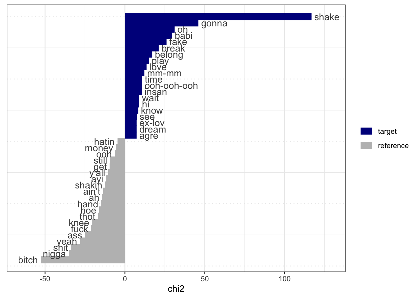
Similar to what we would have inferred from the TF-IDF graphs. Notice that stemming does not always work as expected. Taylor Swift sings about “shake, shake, shake,” and Megan Thee Stallion sings about “shaking.” However, these still appear as distinct features for the two artists.
2.5 Word Frequency Across Artist
We can do something similar to what we did last week to look at word frequencies. Rather than creating a dfm, we can use the dataset as is and extract some basic information—for example, the average number of tokens by artist.
sample_lyrics %>%
  # Tokenize the cleaned lyrics into one-token-per-row (similar in spirit to quanteda tokenization)
  unnest_tokens(word, lyrics_clean) %>%
  # Count tokens per song
  group_by(song) %>%
  mutate(total_tk_song = n()) %>%
  # Keep one row per song (with its token count)
  distinct(song, .keep_all = TRUE) %>%
  # Compute the mean tokens per song within each artist
  group_by(artist) %>%
  mutate(mean_tokens = mean(total_tk_song)) %>%
  # Plot token counts per song, faceted by artist
  ggplot(aes(x = song, y = total_tk_song, fill = artist, color = artist)) +
  geom_col(alpha = 0.8) +
  # Add a dashed line for each artist's mean token count
  geom_hline(aes(yintercept = mean_tokens, color = artist), linetype = "dashed") +
  scale_color_manual(values = wes_palette("Royal2")) +
  scale_fill_manual(values = wes_palette("Royal2")) +
  facet_wrap(~artist, scales = "free_x", nrow = 1) +
  theme_minimal() +
  theme(
    legend.position = "none",
    axis.text.x = element_text(angle = 90, size = 5, vjust = 0.5, hjust = 1)
  ) +
  labs(
    x = "",
    y = "Total Tokens",
    color = "",
    fill = "",
    caption = "Note: Dashed line shows the mean token count by artist."
  )
## group_by: one grouping variable (song)
## mutate (grouped): new variable 'total_tk_song' (integer) with 20 unique values and 0% NA
## distinct (grouped): removed 8,958 rows (>99%), 21 rows remaining (removed 0 groups, 21 groups remaining)
## group_by: one grouping variable (artist)
## mutate (grouped): new variable 'mean_tokens' (double) with 4 unique values and 0% NA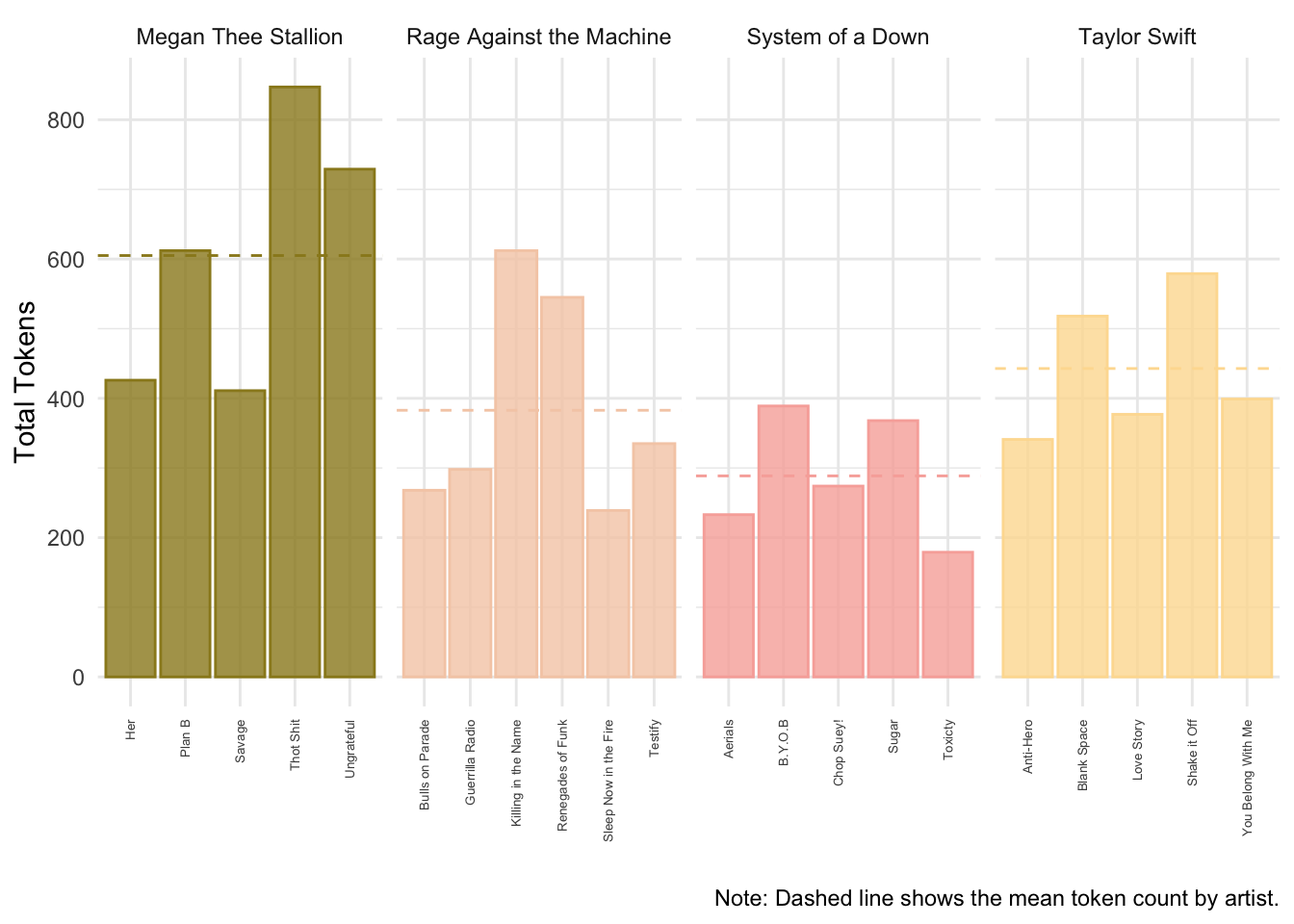
Alternatively, we can estimate the frequency of a specific token by song.
lyrics_totals <- sample_lyrics %>%
  # take the column lyrics_clean and divide it by words
  # this uses a similar tokenizer to quanteda
  unnest_tokens(word, lyrics_clean) %>%
  group_by(song) %>%
  mutate(total_tk_song = n()) %>%
  distinct(song,.keep_all=T)
## group_by: one grouping variable (song)
## mutate (grouped): new variable 'total_tk_song' (integer) with 20 unique values and 0% NA
## distinct (grouped): removed 8,958 rows (>99%), 21 rows remaining (removed 0 groups, 21 groups remaining)
# let's look for "like"
lyrics_like <- sample_lyrics %>%
  # take the column lyrics_clean and divide it by words
  # this uses a similar tokenizer to quanteda
  unnest_tokens(word, lyrics_clean) %>%
  filter(word=="like") %>%
  group_by(song) %>%
  mutate(total_like_song = n()) %>%
  distinct(song,total_like_song)
## filter: removed 8,934 rows (99%), 45 rows remaining
## group_by: one grouping variable (song)
## mutate (grouped): new variable 'total_like_song' (integer) with 7 unique values and 0% NA
## distinct (grouped): removed 33 rows (73%), 12 rows remaining (removed 0 groups, 12 groups remaining)We can now join these two data frames together with the left_join() function using the “song” column as the key. We can then pipe the joined data into a plot.
lyrics_totals %>%
  left_join(lyrics_like, by = "song") %>%
  ungroup() %>%
  mutate(like_prop = total_like_song/total_tk_song) %>%
  ggplot(aes(x=song,y=like_prop,fill=artist,color=artist)) +
  geom_col(alpha=.8) +
  scale_color_manual(values = wes_palette("Royal2")) +
  scale_fill_manual(values = wes_palette("Royal2")) +
  facet_wrap(~artist, scales = "free_x", nrow = 1) +
  theme_minimal() +
  theme(legend.position="none",
        axis.text.x = element_text(angle = 90, size = 5,vjust = 0.5, hjust=1)) +
  labs(x="", y = "Prop. of \'Like\'", color = "", fill = "")
## left_join: added one column (total_like_song)
## > rows only in x 9
## > rows only in lyrics_like ( 0)
## > matched rows 12
## > ====
## > rows total 21
## ungroup: no grouping variables remain
## mutate: new variable 'like_prop' (double) with 13 unique values and 43% NA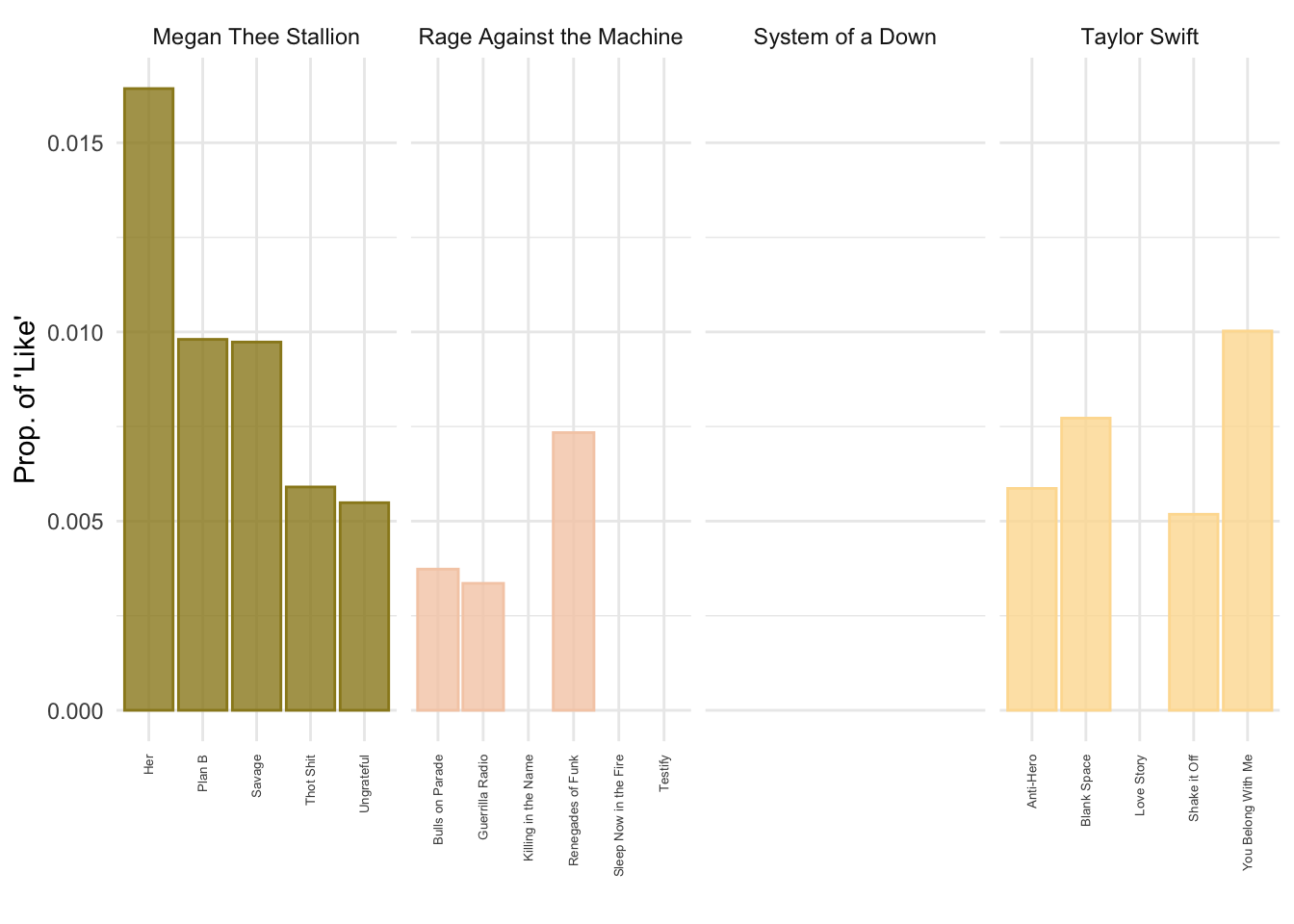
2.6 Final Words
As will often be the case, we won’t be able to cover every single feature that the different packages have to offer, show every object we create, or explore everything we can do with them. My advice is that you go home and explore the code in detail. Try applying it to a different corpus and come to the next class with questions (or just show off what you were able to do).