5 Week 5: Scaling Techniques (Unsupervised Learning I)

Slides

• 6 Scaling Techniques and Topic Modeling (link to slides)

5.1 Setup

As always, we first load the packages that we’ll be using:

library(tidyverse) # for wrangling data
library(tidylog) # to know what we are wrangling
library(tidytext) # for 'tidy' manipulation of text data
library(quanteda) # tokenization power house
library(quanteda.textmodels)
library(wesanderson) # to prettify

5.2 Wordfish

Slapin and Proksch (2008) propose an unsupervised scaling model that places texts on a one-dimensional scale. The underlying assumption is that

\[w_{ik} \sim \text{Poisson}(\lambda_{ik})\] \[\lambda_{ik} = \exp(\alpha_i + \psi_k + \beta_k \times \theta_i)\]

Here, \(\lambda_{ik}\) is generated by \(\alpha_i\) (the “loquaciousness” of politician \(i\), or document fixed effects), \(\psi_k\) (the baseline frequency of word \(k\)), \(\beta_k\) (the discrimination parameter of word \(k\)), and—most importantly, \(\theta_i\) (the politician’s ideological position). Let’s believe, for a moment, that the peer-review system works and use the textmodel_wordfish() function to estimate the ideological positions of U.S. presidents using their inaugural speeches.

us_pres <- readxl::read_xlsx(path = "data/inaugTexts.xlsx")
head(us_pres)

## # A tibble: 6 × 4
##   inaugSpeech               Year President party
##   <chr>                    <dbl> <chr>     <chr>
## 1 "My Countrymen, It a re…  1853 Pierce    Demo…
## 2 "Fellow citizens, I app…  1857 Buchanan  Demo…
## 3 "Fellow-Citizens of the…  1861 Lincoln   Repu…
## 4 "Fellow-Countrymen:\r\n…  1865 Lincoln   Repu…
## 5 "Citizens of the United…  1869 Grant     Repu…
## 6 "Fellow-Citizens:\r\n\r…  1873 Grant     Repu…

The text is pretty clean, so we can convert it into a corpus object, then into a dfm, and apply textmodel_wordfish():

corpus_us_pres <- corpus(us_pres,
                     text_field = "inaugSpeech",
                     unique_docnames = TRUE)

summary(corpus_us_pres)

## Corpus consisting of 41 documents, showing 41 documents:
## 
##    Text Types Tokens Sentences Year
##   text1  1164   3631       104 1853
##   text2   944   3080        89 1857
##   text3  1074   3992       135 1861
##   text4   359    774        26 1865
##   text5   484   1223        40 1869
##   text6   551   1469        43 1873
##   text7   830   2698        59 1877
##   text8  1020   3206       111 1881
##   text9   675   1812        44 1885
##  text10  1351   4720       157 1889
##  text11   821   2125        58 1893
##  text12  1231   4345       130 1897
##  text13   854   2437       100 1901
##  text14   404   1079        33 1905
##  text15  1437   5822       158 1909
##  text16   658   1882        68 1913
##  text17   548   1648        59 1917
##  text18  1168   3717       148 1921
##  text19  1220   4440       196 1925
##  text20  1089   3855       158 1929
##  text21   742   2052        85 1933
##  text22   724   1981        96 1937
##  text23   525   1494        68 1941
##  text24   274    619        27 1945
##  text25   780   2495       116 1949
##  text26   899   2729       119 1953
##  text27   620   1883        92 1957
##  text28   565   1516        52 1961
##  text29   567   1697        93 1965
##  text30   742   2395       103 1969
##  text31   543   1978        68 1973
##  text32   527   1364        52 1977
##  text33   902   2772       129 1981
##  text34   924   2897       124 1985
##  text35   795   2667       141 1989
##  text36   642   1833        81 1993
##  text37   772   2423       111 1997
##  text38   620   1804        97 2001
##  text39   773   2321       100 2005
##  text40   937   2667       110 2009
##  text41   814   2317        88 2013
##     President      party
##        Pierce   Democrat
##      Buchanan   Democrat
##       Lincoln Republican
##       Lincoln Republican
##         Grant Republican
##         Grant Republican
##         Hayes Republican
##      Garfield Republican
##     Cleveland   Democrat
##      Harrison Republican
##     Cleveland   Democrat
##      McKinley Republican
##      McKinley Republican
##   T Roosevelt Republican
##          Taft Republican
##        Wilson   Democrat
##        Wilson   Democrat
##       Harding Republican
##      Coolidge Republican
##        Hoover Republican
##  FD Roosevelt   Democrat
##  FD Roosevelt   Democrat
##  FD Roosevelt   Democrat
##  FD Roosevelt   Democrat
##        Truman   Democrat
##    Eisenhower Republican
##    Eisenhower Republican
##       Kennedy   Democrat
##       Johnson   Democrat
##         Nixon Republican
##         Nixon Republican
##        Carter   Democrat
##        Reagan Republican
##        Reagan Republican
##          Bush Republican
##       Clinton   Democrat
##       Clinton   Democrat
##          Bush Republican
##          Bush Republican
##         Obama   Democrat
##         Obama   Democrat

# We do the whole tokenization sequence
toks_us_pres <- tokens(corpus_us_pres,
                   remove_numbers = TRUE, # Thinks about this
                   remove_punct = TRUE, # Remove punctuation!
                   remove_url = TRUE) # Might be helpful

toks_us_pres <- tokens_remove(toks_us_pres,
                              # Should we though? See Denny and Spirling (2018)
                              c(stopwords(language = "en")),
                              padding = F)

toks_us_pres <- tokens_wordstem(toks_us_pres, language = "en")

dfm_us_pres <- dfm(toks_us_pres)

wfish_us_pres <- textmodel_wordfish(dfm_us_pres, dir = c(28,30)) #Does not really matter what the starting values are, they just serve as anchors for the relative position of the rest of the texts. In this case, I chose Kennedy and Nixon.  
summary(wfish_us_pres)

## 
## Call:
## textmodel_wordfish.dfm(x = dfm_us_pres, dir = c(28, 30))
## 
## Estimated Document Positions:
##           theta      se
## text1  -0.95665 0.03617
## text2  -1.27089 0.03410
## text3  -1.40939 0.02859
## text4  -0.37234 0.08905
## text5  -1.19393 0.05613
## text6  -0.98790 0.05745
## text7  -1.25066 0.03678
## text8  -1.15849 0.03504
## text9  -1.06976 0.04863
## text10 -1.37040 0.02598
## text11 -1.09564 0.04334
## text12 -1.36373 0.02715
## text13 -0.96928 0.04390
## text14  0.14923 0.07992
## text15 -1.67179 0.01837
## text16  0.04315 0.05968
## text17 -0.14887 0.06481
## text18 -0.23081 0.04050
## text19 -0.64288 0.03619
## text20 -0.81708 0.03635
## text21 -0.26568 0.05470
## text22  0.26552 0.05564
## text23  0.56605 0.06544
## text24  0.82801 0.09576
## text25  0.09672 0.04999
## text26  0.37474 0.04777
## text27  0.60860 0.05653
## text28  0.92076 0.05652
## text29  0.96033 0.05604
## text30  1.42553 0.03773
## text31  0.93186 0.05098
## text32  0.87530 0.06217
## text33  1.13366 0.04085
## text34  1.19922 0.03746
## text35  1.25258 0.03978
## text36  1.38319 0.04373
## text37  1.38027 0.03681
## text38  0.87024 0.05416
## text39  0.74125 0.04862
## text40  1.18890 0.03947
## text41  1.05104 0.04446
## 
## Estimated Feature Scores:
##      countrymen  relief    feel   heart    can
## beta    -0.5492 -0.9578 -0.4907 0.80563 0.1395
## psi     -0.5455 -1.8436 -0.3948 0.08719 2.1154
##        know  person  regret    bitter  sorrow
## beta 0.9421 -0.1118 -0.2535  0.003517  0.5177
## psi  0.6955 -0.1544 -2.8010 -2.019466 -2.0333
##         born   posit suitabl  other    rather
## beta  0.7627 -0.9822  -4.124 0.3934  0.005341
## psi  -0.8260 -1.2127  -6.138 0.1718 -0.591945
##        desir circumst   call    limit    period
## beta -0.6215  -0.6367 0.3746 -0.07383 -0.004653
## psi  -0.5405  -1.3629 0.5610 -0.02468 -1.040491
##      presid destini   republ    fill profound
## beta 0.4892  0.2600 -0.27116  0.6825 -0.05042
## psi  0.4727 -0.2598  0.08107 -1.6843 -1.52207
##         sens respons     noth    like shrink
## beta -0.1159  0.2266 -0.08426 0.01539  0.169
## psi  -0.2338  0.8392 -0.25097 0.19869 -1.708

Let’s see whether this makes any sense. Since we know each president’s party, we would expect Republican presidents to cluster together and separate from Democrats (or something along those lines):

# Get predictions:
wfish_preds <- predict(wfish_us_pres, interval = "confidence")

# Tidy everything up:
posi_us_pres <- data.frame(docvars(corpus_us_pres),
                      wfish_preds$fit) %>%
  arrange(fit)

# Plot
posi_us_pres %>%
  ggplot(aes(x = fit, y = reorder(President,fit), xmin = lwr, xmax = upr, color = party)) +
  geom_point(alpha = 0.8) +
  geom_errorbarh(height = 0) +
  labs(x = "Position", y = "", color = "Party") +
  scale_color_manual(values = wes_palette("BottleRocket2")) +
  theme_minimal() +
  ggtitle("Estimated Positions")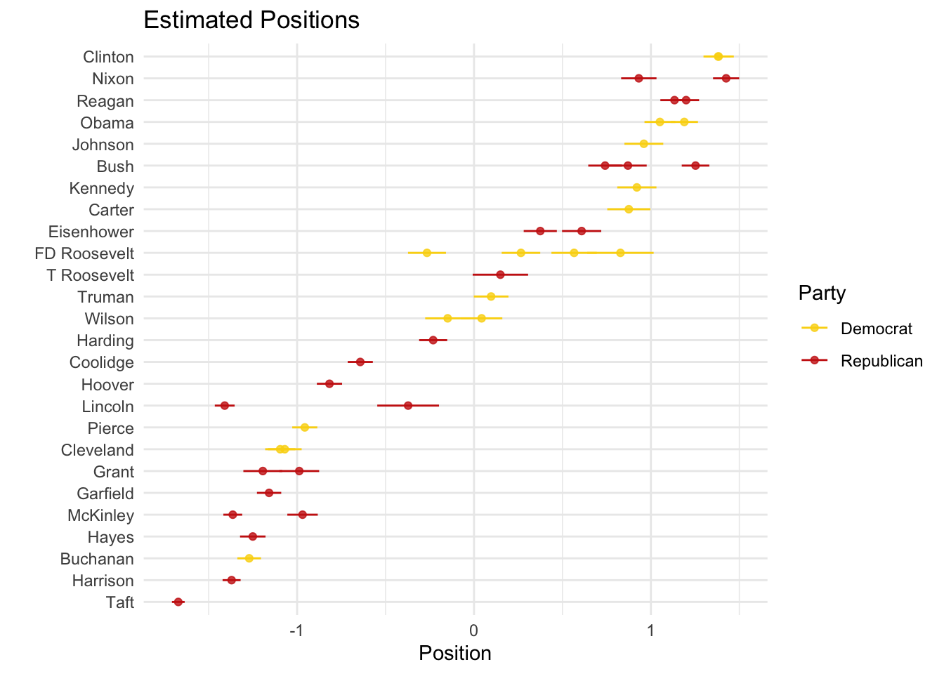

## Warning: `geom_errorbarh()` was deprecated in ggplot2
## 4.0.0.
## ℹ Please use the `orientation` argument of
##   `geom_errorbar()` instead.
## This warning is displayed once per session.
## Call `lifecycle::last_lifecycle_warnings()` to
## see where this warning was generated.

## `height` was translated to `width`.

Two things to note. First, the direction of the scale is a theoretically grounded decision that the researcher has to make (not the algorithm). In our case, based on these results, we could interpret positive values as more left-leaning and negative values as more right-leaning. For visualization purposes, we can flip the direction simply by multiplying by -1:

# Plot inverse
posi_us_pres %>%
  ggplot(aes(x = -fit, y = reorder(President,fit), xmin = -lwr, xmax = -upr, color = party)) +
  geom_point(alpha = 0.8) +
  geom_errorbarh(height = 0) +
  labs(x = "Position", y = "", color = "Party") +
  scale_color_manual(values = wes_palette("BottleRocket2")) +
  theme_minimal() +
  ggtitle("Estimated Positions")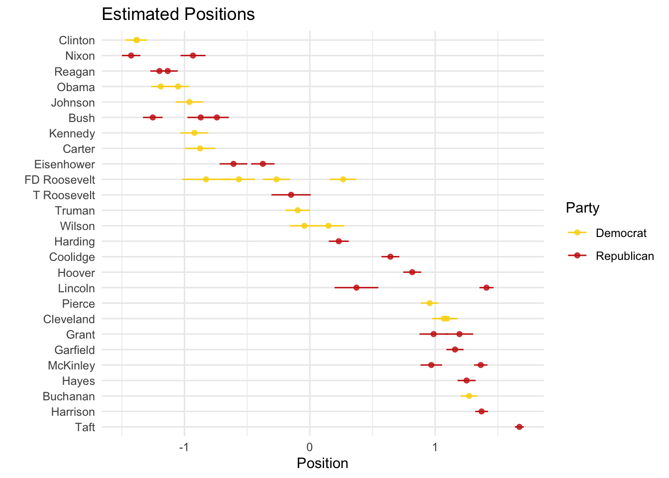

## `height` was translated to `width`.

Second, there seems to be a mismatch between our theoretical expectations and our empirical observations. We might assume that Republicans (Democrats) would talk more similarly to other Republicans (Democrats) and differently from Democrats (Republicans). However, that is not what we see here. What could be happening?

One possibility is that language changes over time, issues change over time, or even what it means to be a Democrat or Republican changes over time. and the model is picking up that temporal shift:

# Plot time
posi_us_pres %>%
  ggplot(aes(y = -fit, x = Year, ymin = -lwr, ymax = -upr, color = party)) +
  geom_point(alpha = 0.8) +
  geom_errorbar() +
  labs(x = "Year", y = "Position", color = "Party") +
  scale_color_manual(values = wes_palette("BottleRocket2")) +
  theme_minimal() +
  ggtitle("Estimated Positions")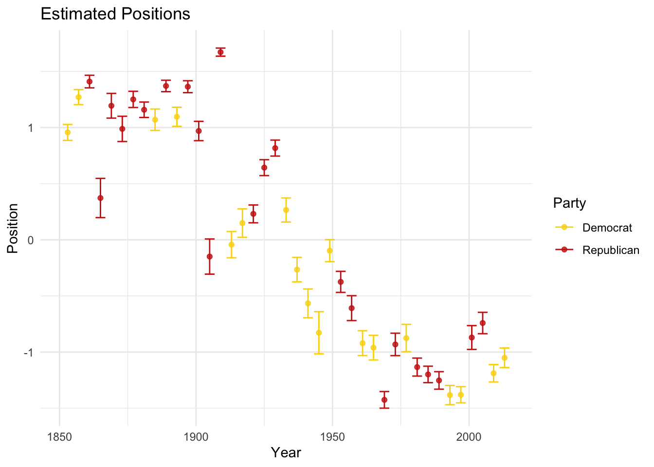

That seems like one possible explanation. Another is that our preprocessing steps substantively modified the texts (see Denny and Spirling 2018). We can estimate the model again using a differently preprocessed version of the text:

# Tokenization only removing punctuation
toks_us_pres2 <- tokens(corpus_us_pres,
                   remove_punct = TRUE) 

dfm_us_pres2 <- dfm(toks_us_pres2)
wfish_us_pres <- textmodel_wordfish(dfm_us_pres2, dir = c(28,30))  

# Get predictions:
wfish_preds <- predict(wfish_us_pres, interval = "confidence")

# Tidy everything up:
posi_us_pres <- data.frame(docvars(corpus_us_pres),
                      wfish_preds$fit) %>%
  arrange(fit)

# Plot
posi_us_pres %>%
  ggplot(aes(x = -fit, y = reorder(President,fit), xmin = -lwr, xmax = -upr, color = party)) +
  geom_point(alpha = 0.8) +
  geom_errorbarh(height = 0) +
  labs(x = "Position", y = "", color = "Party") +
  scale_color_manual(values = wes_palette("BottleRocket2")) +
  theme_minimal() +
  ggtitle("Estimated Positions (Minimal Pre-Processing)")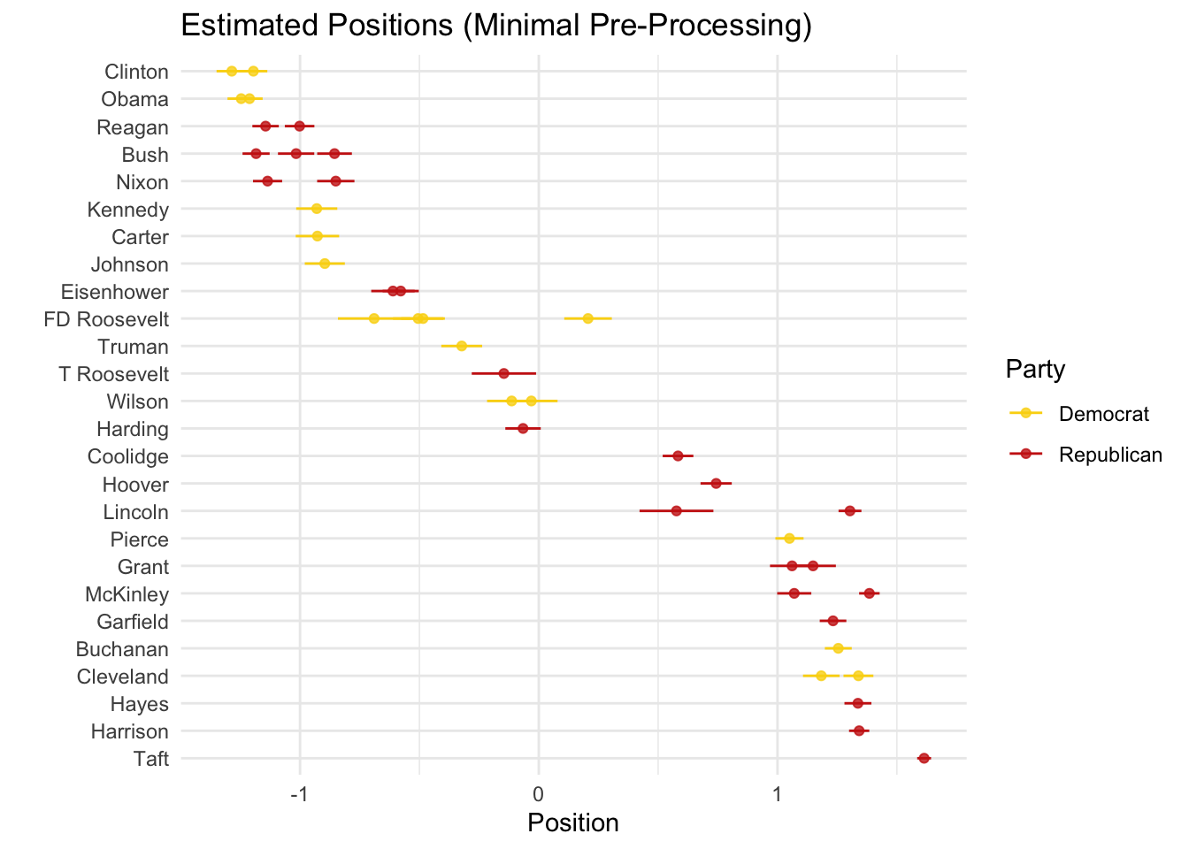

## `height` was translated to `width`.

At the very least, the within president differences in estimates have narrowed, but time seems to still be the best predictor:

# Plot time
posi_us_pres %>%
  ggplot(aes(y = -fit, x = Year, ymin = -lwr, ymax = -upr, color = party)) +
  geom_point(alpha = 0.8) +
  geom_errorbar() +
  labs(x = "Year", y = "Position", color = "Party") +
  scale_color_manual(values = wes_palette("BottleRocket2")) +
  theme_minimal() +
  ggtitle("Estimated Positions (Minimal Pre-Processing)")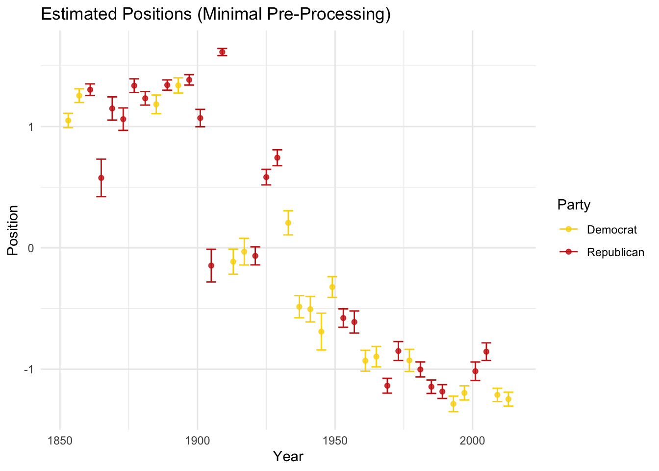

If time is the main predictor, then we may need to focus on periods that are more comparable across parties (e.g., the era after the Civil Rights Act).

5.3 Homework 2:

1. We had a hard time scaling our text, so we looked at some possible problems. What are possible solutions if we want to position U.S. presidents on an ideological scale using text?
2. Use the data/candidate-tweets.csv data to run an STM. Decide what your covariates are going to be. Decide whether you will use all the data or a sample of the data. Decide whether you are going to aggregate or split the text in some way (i.e., decide your unit of analysis). Decide the number of topics you will look for (try more than one option). What can you tell me about the topics tweeted by the 2015 U.S. primary candidates?
3. Choose three topics (see Week 6). Can you place the candidates on an ideological scale within each topic (determine the \(\theta\) threshold for when you can say that a tweet is mostly about a topic)? Does it make sense? Why or why not?