15 Lecture 6: The Multiple Regression Model I

Slides

• 7 The Multiple Regression Model (link)

15.1 Introduction

We continue studying the simple regression model.

Figure 15.1: Slides for 7 The Multiple Regression Model.

15.2 Vignette 6.1

Once again, let’s simulate some data. Maybe we are interested in urban and rural towns (70% are urban) :

df <- tibble(urban = sample(c(0,1),500,replace=T,prob=c(.3,.7))) %>%
  ## Urban towns spend, on average, $3 million more on wages than rural towns
  mutate(expen_wages = 3*urban+runif(500,min=0,max=4)) %>%
  ## Urban towns are also have greater incomes (e.g., from taxes), but these are reduced by their high wage expenditures:
  mutate(log_income = 1 + 2*urban - .3*expen_wages + rnorm(500,mean=2)) ## <- Population Eq.

Now we can estimate the effect of wage expenditure on income:

model_a <- lm(log_income ~ expen_wages, data = df) 
summary(model_a) 

## 
## Call:
## lm(formula = log_income ~ expen_wages, data = df)
## 
## Residuals:
##     Min      1Q  Median      3Q     Max 
## -4.2103 -0.8477 -0.0097  0.8111  4.4946 
## 
## Coefficients:
##             Estimate Std. Error t value
## (Intercept)  2.60611    0.13465   19.35
## expen_wages  0.11076    0.03027    3.66
##             Pr(>|t|)    
## (Intercept)  < 2e-16 ***
## expen_wages 0.000279 ***
## ---
## Signif. codes:  
## 0 '***' 0.001 '**' 0.01 '*' 0.05 '.' 0.1 ' ' 1
## 
## Residual standard error: 1.243 on 498 degrees of freedom
## Multiple R-squared:  0.02619,    Adjusted R-squared:  0.02424 
## F-statistic: 13.39 on 1 and 498 DF,  p-value: 0.0002794

Wait what? (Interpret a log ~ level)

15.3 Vignette 6.2

Let’s see… How can we remove everything from wages that is explained by urban? How can we remove everything from income that is explained by urban?

df %>% group_by(urban) %>%
  summarise(income_urb= mean(log_income)) 

## summarise: now 2 rows and 2 columns, ungrouped

## # A tibble: 2 × 2
##   urban income_urb
##   <dbl>      <dbl>
## 1     0       2.26
## 2     1       3.45

df %>% group_by(urban) %>% 
  summarise(expen_wages_urb = mean(expen_wages))

## summarise: now 2 rows and 2 columns, ungrouped

## # A tibble: 2 × 2
##   urban expen_wages_urb
##   <dbl>           <dbl>
## 1     0            2.06
## 2     1            5.04

The difference between what is explained by urban of income/expendinture (mean) and the observed value of income/expenditure is…

df <- df %>% group_by(urban) %>%
  mutate(log_income_residual = log_income - mean(log_income),
         expen_wages_residual = expen_wages - mean(expen_wages)) %>%
  ungroup()

## ungroup: no grouping variables remain

The residual… what is not explained by urban!!

model_b <- lm(log_income_residual ~ expen_wages_residual, data = df) 
summary(model_b) ### CLOSER!

## 
## Call:
## lm(formula = log_income_residual ~ expen_wages_residual, data = df)
## 
## Residuals:
##     Min      1Q  Median      3Q     Max 
## -3.0437 -0.7391  0.0019  0.7239  3.4277 
## 
## Coefficients:
##                        Estimate Std. Error
## (Intercept)          -9.089e-17  4.790e-02
## expen_wages_residual -2.971e-01  4.051e-02
##                      t value Pr(>|t|)    
## (Intercept)            0.000        1    
## expen_wages_residual  -7.335 9.04e-13 ***
## ---
## Signif. codes:  
## 0 '***' 0.001 '**' 0.01 '*' 0.05 '.' 0.1 ' ' 1
## 
## Residual standard error: 1.071 on 498 degrees of freedom
## Multiple R-squared:  0.09751,    Adjusted R-squared:  0.0957 
## F-statistic: 53.81 on 1 and 498 DF,  p-value: 9.037e-13

Let’s plot:

A <- ggplot(df, aes(x=expen_wages,y=log_income)) +
  geom_point() +
  labs(title = "0. Relation between wages and income. Beta = 0.13") +
  geom_smooth(method = "lm") +
  xlim(c(-3,7)) + ylim(c(-3,6))
A

## `geom_smooth()` using formula = 'y ~ x'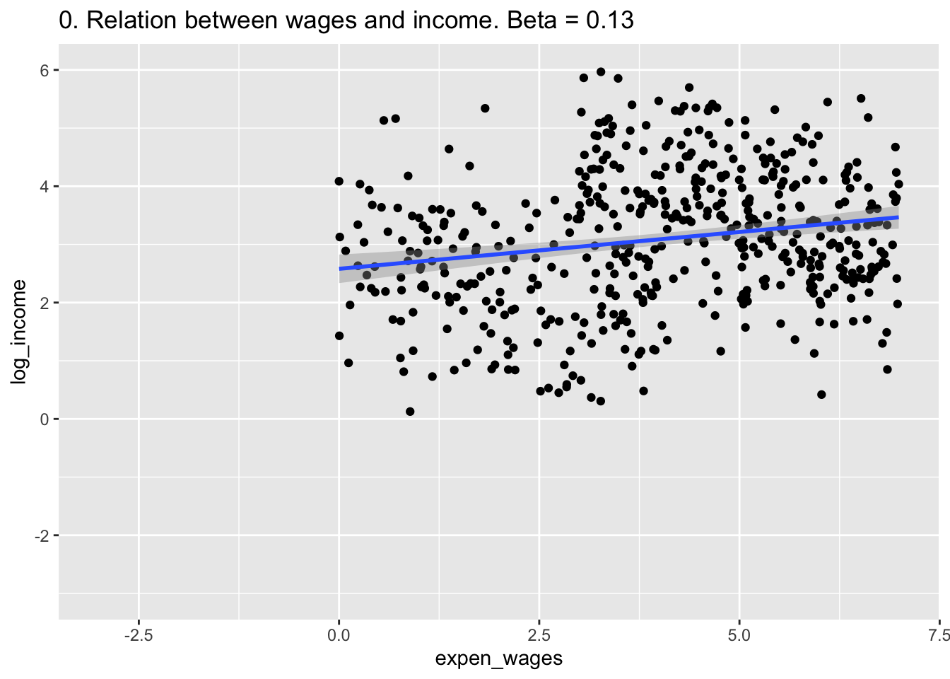

B <- ggplot(df, aes(x=expen_wages,y=log_income,color = factor(urban))) +
  geom_point() +
  labs(title = "1. Relation between wages and income divided by urban.") +
  xlim(c(-3,7)) + ylim(c(-3,6))
B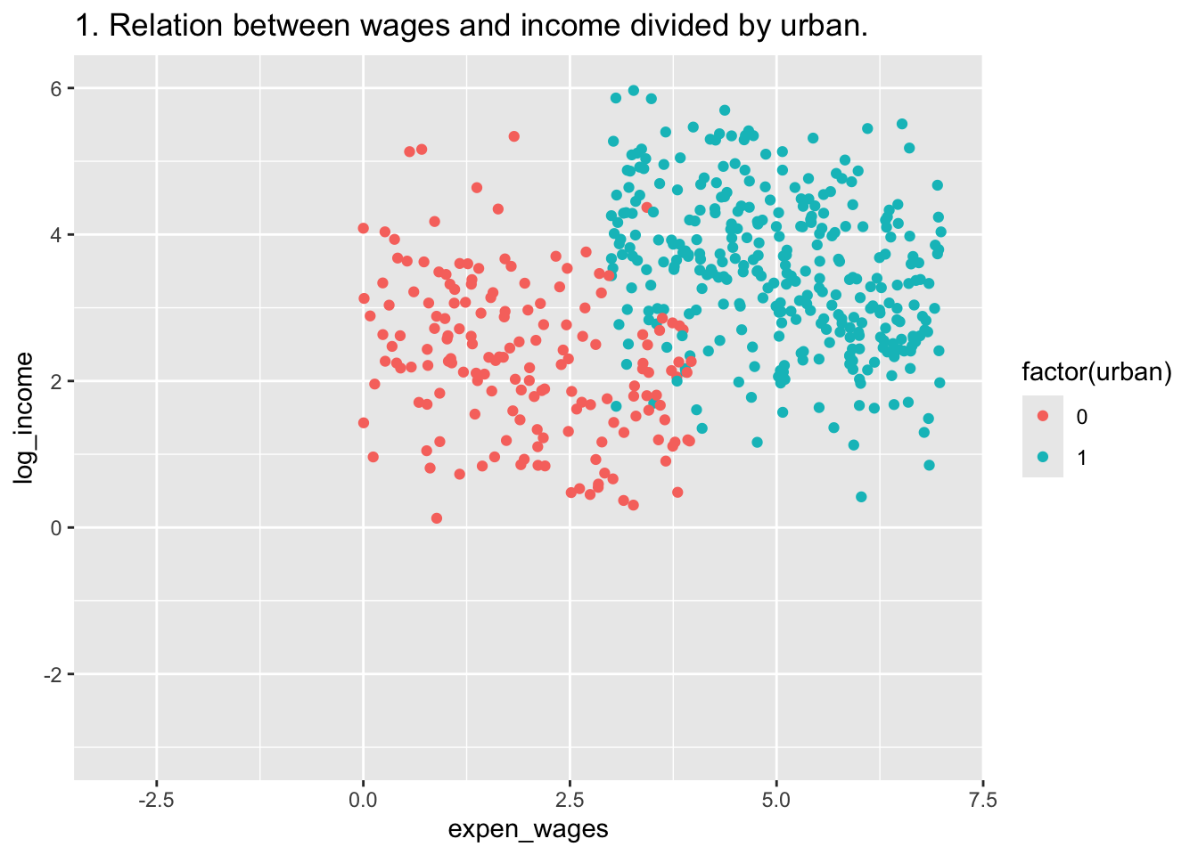

C <- ggplot(df, aes(x=expen_wages_residual,y=log_income,color = factor(urban))) +
  geom_point() +
  labs(title = "2. We remove the difference of wages explained by urban.")+
  xlim(c(-3,7)) + ylim(c(-3,6))
C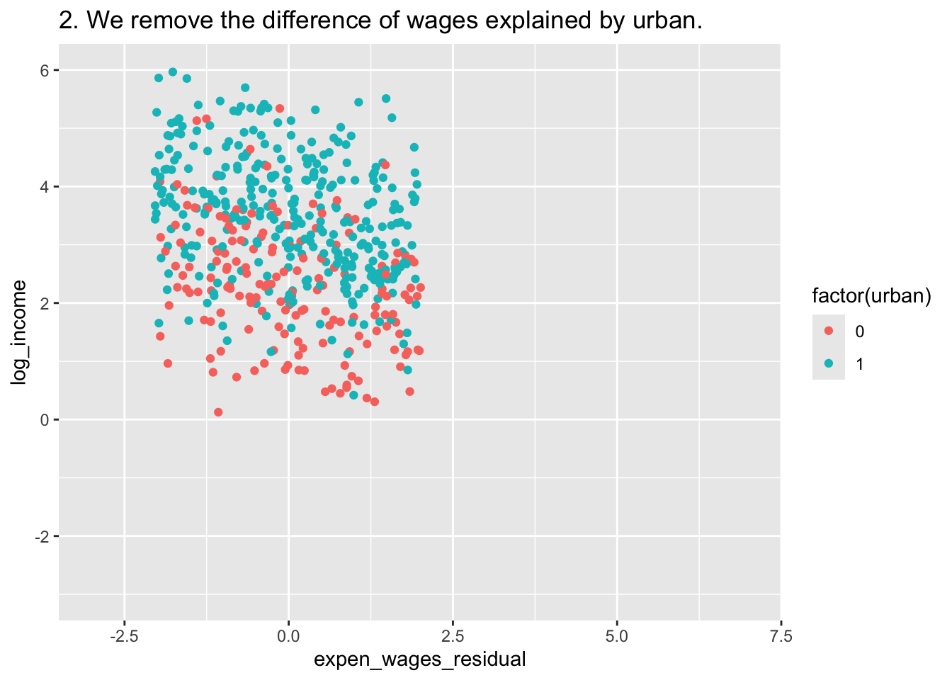

D <- ggplot(df, aes(x=expen_wages_residual,y=log_income_residual,color = factor(urban))) +
  geom_point() +
  labs(title = "3. We remove the difference of income explained by urban.")+
  xlim(c(-3,7)) + ylim(c(-3,6))
D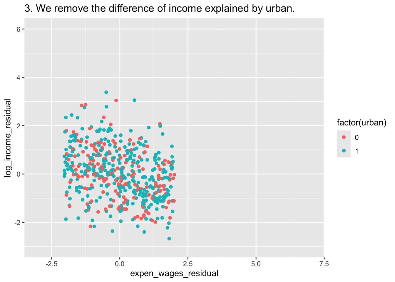

E <- ggplot(df, aes(expen_wages_residual,y=log_income_residual)) +
  geom_point() +
  labs(title = "4. We analize what is left. Beta = -0.22") +
  geom_smooth(method = "lm")+
  xlim(c(-3,7)) + ylim(c(-3,6))
E

## `geom_smooth()` using formula = 'y ~ x'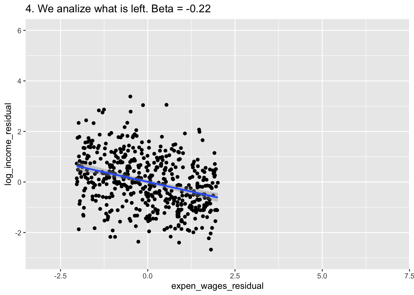

ggarrange(A,B,C,D,E,
          common.legend = T,
          ncol = 2,
          nrow = 3)

## `geom_smooth()` using formula = 'y ~ x'
## `geom_smooth()` using formula = 'y ~ x'
## `geom_smooth()` using formula = 'y ~ x'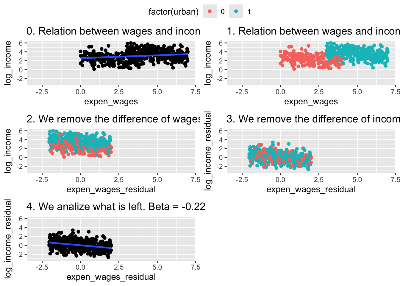

15.4 Lecture Assignment

1. Using simulated data (or any other approach, including replication from a paper), show the effects of high collinearity, multicollinearity, and perfect collinearity on the estimates from OLS models.

2. What are the theoretical implications from models with high collinearity, multicollinearity, and perfect collinearity? What are possible solutions to high collinearity, multicollinearity, and perfect collinearity?