Chapter 22 Lecture 9: Interactions | PS9591: Regressions and Causal Inference

Slides

10 Interactions (link)

Figure 22.1: Slides for 10 Interactions.

22.1 Interactions in Linear Models

Interactions let the effect of one variable depend on the level of another. In social science language: context conditions the relationship.

We will build intuition with two vignettes:

State-level turnout (OLS): We’ll also compare classical vs robust standard errors.
Individual voting (LPM): We’ll use a linear probability model to keep interpretation simple, and then discuss trade-offs.

Start with a model with an interaction:

\[ y = \beta_0 + \beta_1 X + \beta_2 Z + \beta_3 (X\cdot Z) + \varepsilon \]

Two key interpretations:

Conditional effect of \(X\) (a.k.a. “simple slope”): \[ \frac{\partial E[y]}{\partial X} = \beta_1 + \beta_3 Z \]
Conditional regression line:

If \(Z=0\): \(E[y|X,Z=0] = \beta_0 + \beta_1 X\)
If \(Z=1\): \(E[y|X,Z=1] = (\beta_0+\beta_2) + (\beta_1+\beta_3)X\)

So, \(\beta_3\) is literally the difference in slopes (when \(Z\) is a dummy).

We’ll plug in real coefficients below.

22.2 Vignette A: Turnout and conditional relationships (OLS)

library(tidyverse)
library(sjPlot)
library(marginaleffects)
library(modelsummary)

data(election_turnout, package = "stevedata")

election_turnout <- election_turnout %>%
  mutate(
    ss = factor(ss),
    trumpw = factor(trumpw),
    region = factor(region),
    gdppercap_ln = log(gdppercap)
  )

summary(election_turnout$turnoutho)

##    Min. 1st Qu.  Median    Mean 3rd Qu.    Max. 
##   42.20   56.75   60.90   60.82   64.75   74.20

sd(election_turnout$turnoutho)

## [1] 6.117199

22.2.1 A.1 Main example (continuous × dummy): education and swing states

Here is the interaction model:

\[ turnoutho_i = \beta_0 + \beta_1 percoled_i + \beta_2 ss_i + \beta_3(percoled_i \cdot ss_i) + \varepsilon_i \]

model_turnout_cd <- lm(
  turnoutho ~ percoled*ss + gdppercap_ln + trumpw,
  data = election_turnout
)

# Side-by-side: classical vs robust SEs
modelsummary(
  list("Classical SEs" = model_turnout_cd,
       "Robust SEs (HC3)" = model_turnout_cd),
  vcov = list("Classical SEs" = NULL,
              "Robust SEs (HC3)" = "HC3"),
  title = "Turnout with Interaction: percoled × swing state",
  coef_rename = c(
    "(Intercept)" = "Intercept",
    "percoled" = "% College Educated",
    "ss1" = "Swing State",
    "percoled:ss1" = "% College × Swing State",
    "gdppercap_ln" = "GDP pc (log)",
    "trumpw1" = "Trump Won"
  ),
  gof_map = c("nobs","r.squared"),
  stars = TRUE,
  notes = list(
    "Column 1: classical OLS standard errors. Column 2: robust (HC3) standard errors.",
    "*** p<0.001, ** p<0.01, * p<0.05"
  )
)

Turnout with Interaction: percoled × swing state
	Classical SEs	Robust SEs (HC3)
+ p < 0.1, * p < 0.05, p < 0.01, * p < 0.001
Column 1: classical OLS standard errors. Column 2: robust (HC3) standard errors.
* p<0.001, p<0.01, * p<0.05
Intercept	70.397	70.397
	(41.929)	(56.170)
% College Educated	0.422+	0.422
	(0.225)	(0.282)
Swing State	-0.022	-0.022
	(10.226)	(12.187)
GDP pc (log)	-2.148	-2.148
	(4.280)	(5.070)
Trump Won	-0.522	-0.522
	(1.847)	(2.900)
% College × Swing State	0.239	0.239
	(0.341)	(0.405)
Num.Obs.	51	51
R2	0.447	0.447

From the model:

When ss = 0 (not a swing state), the slope of percoled is: \[ \text{slope} = \beta_1 \]
When ss = 1 (swing state), the slope of percoled is: \[ \text{slope} = \beta_1 + \beta_3 \]

Let’s compute and display these “simple slopes” directly:

# Simple slopes of percoled at ss=0 and ss=1
slopes(model_turnout_cd, variables = "percoled", newdata = datagrid(ss = levels(election_turnout$ss)))

## 
##  ss Estimate Std. Error    z Pr(>|z|)   S
##   0    0.422      0.225 1.87   0.0613 4.0
##   1    0.661      0.342 1.93   0.0535 4.2
##     2.5 % 97.5 %
##  -0.01996  0.863
##  -0.00995  1.332
## 
## Term: percoled
## Type: response
## Comparison: dY/dX

Now let’s plot predicted turnout across percoled for swing vs non-swing states:

plot_model(model_turnout_cd, type = "pred", terms = c("percoled", "ss")) +
  theme_minimal()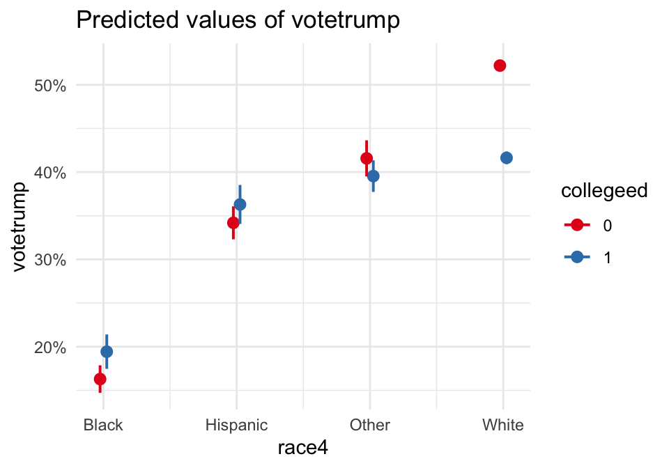

And a marginal effect plot is another way of saying the same thing:

plot_slopes(model_turnout_cd, variables = "percoled", condition = "ss") +
  geom_hline(yintercept = 0, linetype = "dotted") +
  theme_minimal()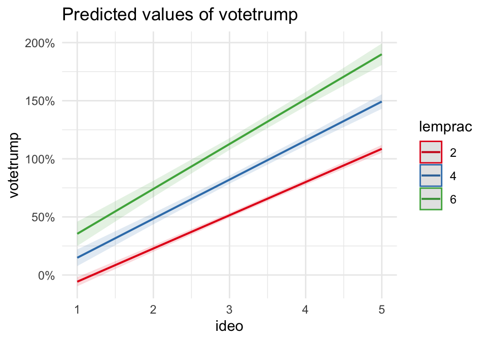

22.2.2 A.2 Interaction zoo (OLS)

22.2.2.1 (1) Dummy × Dummy: swing states × Trump-win states

Now we interpret \(\beta_3\) as a difference-in-differences term:

model_turnout_dd <- lm(
  turnoutho ~ ss*trumpw + percoled + gdppercap_ln,
  data = election_turnout
)

modelsummary(
  model_turnout_dd,
  title = "Turnout: swing state × Trump won (Dummy × Dummy)",
  coef_rename = c(
    "(Intercept)" = "Intercept",
    "ss1" = "Swing State",
    "trumpw1" = "Trump Won",
    "ss1:trumpw1" = "Swing × Trump Won",
    "percoled" = "% College Educated",
    "gdppercap_ln" = "GDP pc (log)"
  ),
  gof_map = c("nobs","r.squared"),
  stars = TRUE
)

Turnout: swing state × Trump won (Dummy × Dummy)
	(1)
+ p < 0.1, * p < 0.05, p < 0.01, * p < 0.001
Intercept	77.523+
	(41.197)
Swing State	6.526*
	(2.495)
Trump Won	-0.848
	(2.069)
% College Educated	0.469*
	(0.215)
GDP pc (log)	-2.911
	(4.176)
Swing × Trump Won	0.908
	(3.258)
Num.Obs.	51
R2	0.442

plot_model(model_turnout_dd, type = "int") +
  theme_minimal()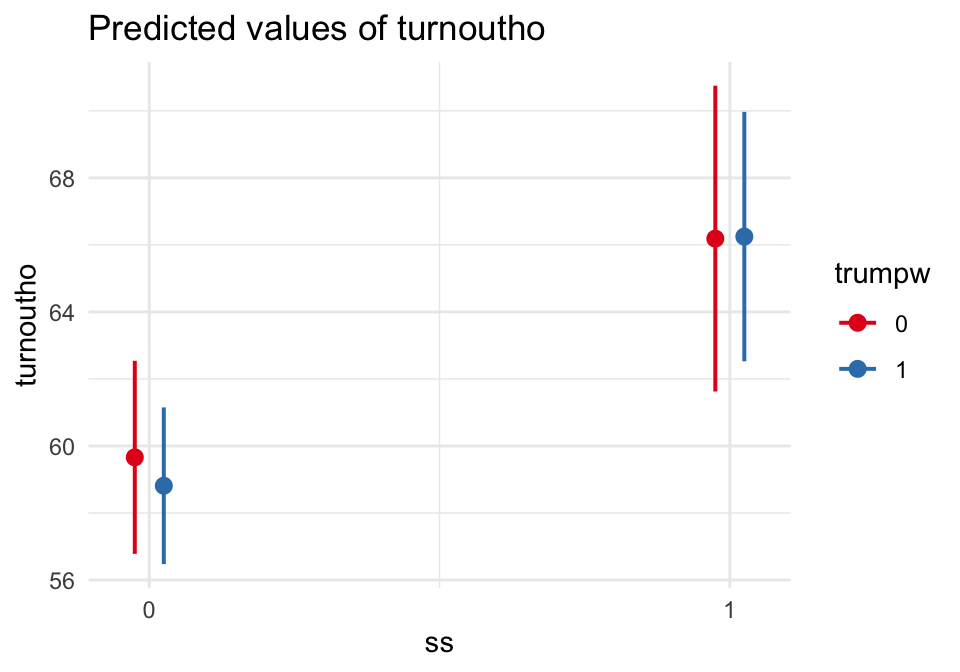

22.2.2.2 (2) Dummy × Categorical: swing states × region

model_turnout_dc <- lm(
  turnoutho ~ ss*region + percoled + gdppercap_ln + trumpw,
  data = election_turnout
)

modelsummary(
  model_turnout_dc,
  title = "Turnout: swing state × region (Dummy × Categorical)",
  gof_map = c("nobs","r.squared"),
  stars = TRUE
)

Turnout: swing state × region (Dummy × Categorical)
	(1)
+ p < 0.1, * p < 0.05, p < 0.01, * p < 0.001
(Intercept)	77.370+
	(42.926)
ss1	7.753**
	(2.807)
regionNortheast	0.386
	(3.016)
regionSouth	-2.758
	(2.229)
regionWest	-2.647
	(2.394)
percoled	0.399+
	(0.225)
gdppercap_ln	-2.547
	(4.335)
trumpw1	-0.986
	(2.126)
ss1 × regionNortheast	-2.447
	(4.846)
ss1 × regionSouth	-1.230
	(4.191)
ss1 × regionWest	-3.241
	(4.705)
Num.Obs.	51
R2	0.512

plot_model(model_turnout_dc, type = "pred", terms = c("region","ss")) +
  theme_minimal()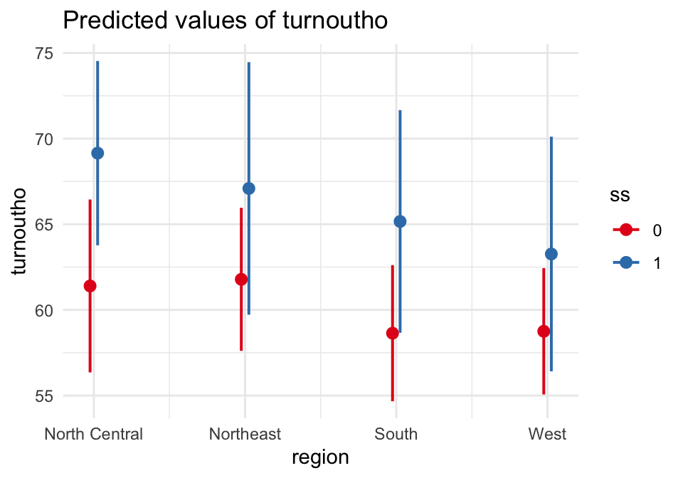

22.2.2.3 (3) Continuous × Continuous: education × state wealth

model_turnout_cc <- lm(
  turnoutho ~ percoled*gdppercap_ln + ss + trumpw,
  data = election_turnout
)

modelsummary(
  model_turnout_cc,
  title = "Turnout: percoled × log(GDP pc) (Continuous × Continuous)",
  coef_rename = c(
    "(Intercept)" = "Intercept",
    "percoled" = "% College Educated",
    "gdppercap_ln" = "GDP pc (log)",
    "percoled:gdppercap_ln" = "% College × GDP pc (log)",
    "ss1" = "Swing State",
    "trumpw1" = "Trump Won"
  ),
  gof_map = c("nobs","r.squared"),
  stars = TRUE
)

Turnout: percoled × log(GDP pc) (Continuous × Continuous)
	(1)
+ p < 0.1, * p < 0.05, p < 0.01, * p < 0.001
Intercept	-101.422
	(89.009)
% College Educated	5.491*
	(2.261)
GDP pc (log)	13.101
	(8.191)
Swing State	6.614***
	(1.540)
Trump Won	0.487
	(1.825)
% College × GDP pc (log)	-0.447*
	(0.201)
Num.Obs.	51
R2	0.497

# Visualize: predicted turnout across percoled at representative GDP values
plot_model(model_turnout_cc, type = "pred",
           terms = c("percoled", "gdppercap_ln [7.5, 8.0, 8.5]")) +
  theme_minimal()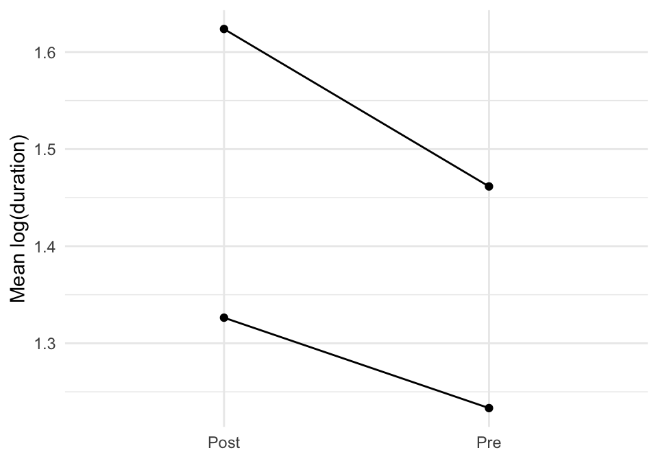

# Marginal effect of percoled across GDP
plot_slopes(model_turnout_cc, variables = "percoled", condition = "gdppercap_ln") +
  geom_hline(yintercept = 0, linetype = "dotted") +
  theme_minimal()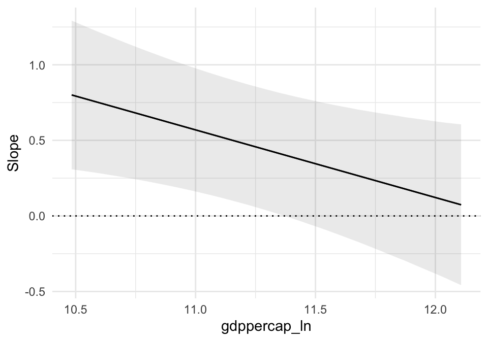

22.3 Vignette B: Interactions in a Linear Probability Model (TV16)

data(TV16, package = "stevedata")

TV16 <- TV16 %>%
  mutate(
    female = factor(female),
    collegeed = factor(collegeed),
    # Collapse race for cleaner teaching plots:
    race4 = case_when(
      racef == "White" ~ "White",
      racef == "Black" ~ "Black",
      racef == "Hispanic" ~ "Hispanic",
      TRUE ~ "Other"
    ),
    race4 = factor(race4),
    votetrump = as.numeric(votetrump)
  )

table(TV16$votetrump)

## 
##     0     1 
## 26177 18755

22.3.1 Sidebar: why an LPM here?

We could model a binary outcome using logit/probit. But for the purposes of this class, the LPM is extremely convenient:

Coefficients are in percentage points (because \(y\in\{0,1\}\)).
Interactions are easy to interpret and visualize with straight lines.
The main statistical downside is heteroskedasticity (so robust SEs are usually a good default).
Another downside is that predicted values can fall outside \([0,1]\). We can check this.

We’ll treat this as a pedagogical model and focus on interpretation.

22.3.2 B.1 Main example (continuous × dummy): ideology × college education

model_tv_cd <- lm(
  votetrump ~ ideo*collegeed + female + race4,
  data = TV16
)

modelsummary(
  list("Classical SEs" = model_tv_cd,
       "Robust SEs (HC3)" = model_tv_cd),
  vcov = list("Classical SEs" = NULL,
              "Robust SEs (HC3)" = "HC3"),
  title = "LPM: Trump vote with interaction (ideo × college)",
  stars = TRUE,
  notes = list(
    "Binary outcome estimated by OLS (Linear Probability Model).",
    "Column 2 uses robust (HC3) standard errors."
  )
)

LPM: Trump vote with interaction (ideo × college)
	Classical SEs	Robust SEs (HC3)
+ p < 0.1, * p < 0.05, p < 0.01, * p < 0.001
Binary outcome estimated by OLS (Linear Probability Model).
Column 2 uses robust (HC3) standard errors.
(Intercept)	-0.575***	-0.575***
	(0.009)	(0.008)
ideo	0.258***	0.258***
	(0.002)	(0.002)
collegeed1	-0.056***	-0.056***
	(0.011)	(0.008)
female1	-0.034***	-0.034***
	(0.004)	(0.004)
race4Hispanic	0.178***	0.178***
	(0.009)	(0.009)
race4Other	0.243***	0.243***
	(0.009)	(0.009)
race4White	0.305***	0.305***
	(0.006)	(0.006)
ideo × collegeed1	-0.008*	-0.008**
	(0.003)	(0.003)
Num.Obs.	43430	43430
R2	0.408	0.408
R2 Adj.	0.407	0.407
AIC	39160.7	39160.7
BIC	39238.8	39238.8
Log.Lik.	-19571.344	-19571.344
RMSE	0.38	0.38
Std.Errors	Classical SEs	Robust SEs (HC3)

When collegeed = 0, the marginal effect of ideology is \(\beta_1\).
When collegeed = 1, the marginal effect is \(\beta_1 + \beta_3\).
Because \(y\) is 0/1, interpret these as percentage point changes in Pr(Trump vote).

plot_slopes(model_tv_cd, variables = "ideo", condition = "collegeed") +
  geom_hline(yintercept = 0, linetype = "dotted") +
  theme_minimal()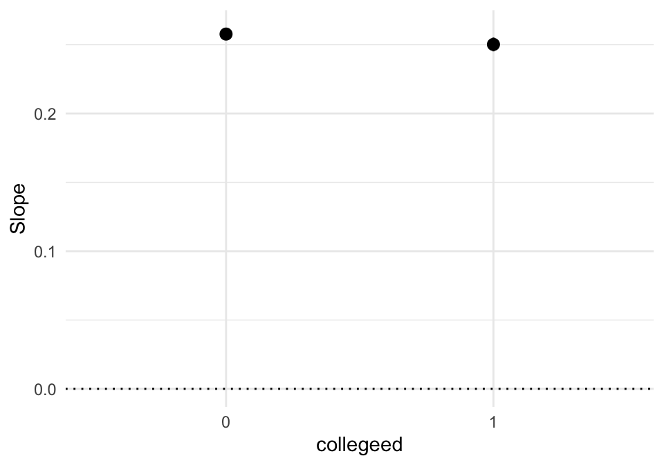

plot_model(model_tv_cd, type = "pred", terms = c("ideo", "collegeed")) +
  theme_minimal() +
  scale_y_continuous(labels = scales::percent)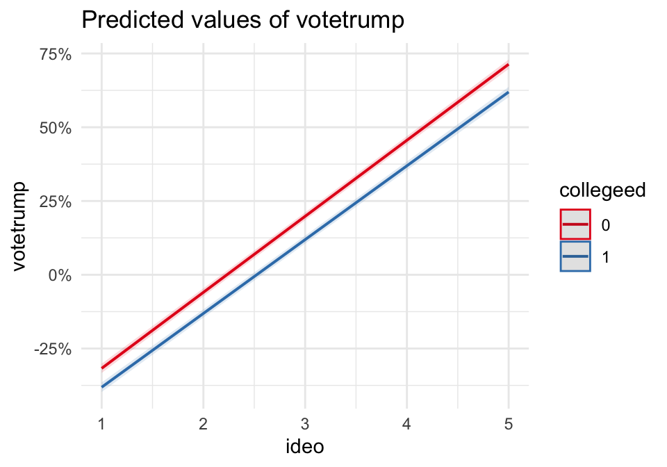

Quick check: do predicted values leave [0,1]?

pred_check <- predictions(model_tv_cd) %>%
  summarize(min_pred = min(estimate), max_pred = max(estimate))
pred_check

##    min_pred max_pred
## 1 -0.415327 1.018627

22.3.3 B.2 Interaction zoo (LPM)

22.3.3.1 (1) Dummy × Dummy: female × college

model_tv_dd <- lm(
  votetrump ~ female*collegeed + ideo + race4,
  data = TV16
)

modelsummary(
  model_tv_dd,
  title = "LPM: female × college (Dummy × Dummy)",
  stars = TRUE
)

LPM: female × college (Dummy × Dummy)
	(1)
+ p < 0.1, * p < 0.05, p < 0.01, * p < 0.001
(Intercept)	-0.562***
	(0.008)
female1	-0.041***
	(0.005)
collegeed1	-0.087***
	(0.005)
ideo	0.255***
	(0.002)
race4Hispanic	0.178***
	(0.009)
race4Other	0.244***
	(0.009)
race4White	0.306***
	(0.006)
female1 × collegeed1	0.016*
	(0.007)
Num.Obs.	43430
R2	0.408
R2 Adj.	0.407
AIC	39161.2
BIC	39239.3
Log.Lik.	-19571.578
RMSE	0.38

plot_model(model_tv_dd, type = "int") +
  theme_minimal() +
  scale_y_continuous(labels = scales::percent)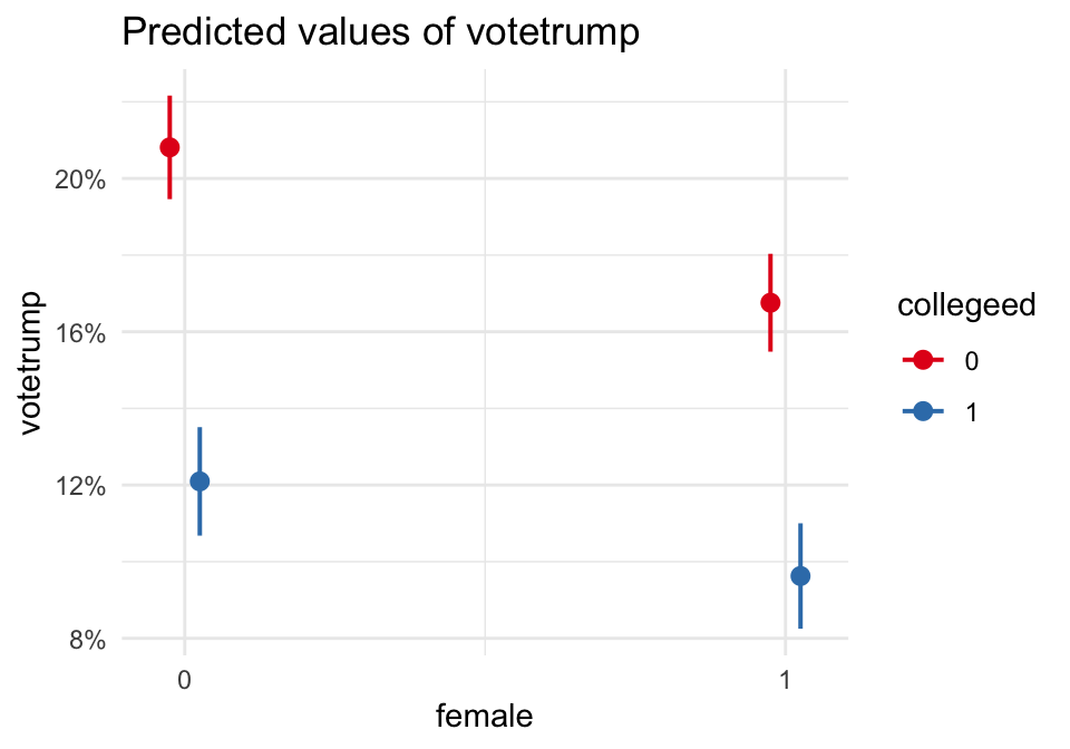

22.3.3.2 (2) Dummy × Categorical: college × race4 (collapsed)

model_tv_dc <- lm(
  votetrump ~ collegeed*race4 + female + ideo,
  data = TV16
)

modelsummary(
  model_tv_dc,
  title = "LPM: college × race4 (Dummy × Categorical)",
  stars = TRUE
)

LPM: college × race4 (Dummy × Categorical)
	(1)
+ p < 0.1, * p < 0.05, p < 0.01, * p < 0.001
(Intercept)	-0.604***
	(0.009)
collegeed1	0.031*
	(0.012)
race4Hispanic	0.179***
	(0.012)
race4Other	0.253***
	(0.013)
race4White	0.359***
	(0.008)
female1	-0.035***
	(0.004)
ideo	0.254***
	(0.002)
collegeed1 × race4Hispanic	-0.010
	(0.019)
collegeed1 × race4Other	-0.052**
	(0.019)
collegeed1 × race4White	-0.137***
	(0.013)
Num.Obs.	43430
R2	0.410
R2 Adj.	0.410
AIC	38986.4
BIC	39081.9
Log.Lik.	-19482.200
RMSE	0.38

plot_model(model_tv_dc, type = "pred", terms = c("race4", "collegeed")) +
  theme_minimal() +
  scale_y_continuous(labels = scales::percent)

22.3.3.3 (3) Continuous × Continuous: ideology × racial resentment proxy (lemprac)

model_tv_cc <- lm(
  votetrump ~ ideo*lemprac + female + collegeed + race4,
  data = TV16
)

modelsummary(
  model_tv_cc,
  title = "LPM: ideo × lemprac (Continuous × Continuous)",
  stars = TRUE
)

LPM: ideo × lemprac (Continuous × Continuous)
	(1)
+ p < 0.1, * p < 0.05, p < 0.01, * p < 0.001
(Intercept)	-0.499***
	(0.008)
ideo	0.236***
	(0.002)
lemprac	0.078***
	(0.012)
female1	-0.023***
	(0.004)
collegeed1	-0.075***
	(0.004)
race4Hispanic	0.161***
	(0.009)
race4Other	0.222***
	(0.009)
race4White	0.285***
	(0.006)
ideo × lemprac	0.025***
	(0.004)
Num.Obs.	43428
R2	0.428
R2 Adj.	0.428
AIC	37647.4
BIC	37734.2
Log.Lik.	-18813.719
RMSE	0.37

plot_model(model_tv_cc, type = "pred", terms = c("ideo", "lemprac [2,4,6]")) +
  theme_minimal() +
  scale_y_continuous(labels = scales::percent)

plot_slopes(model_tv_cc, variables = "ideo", condition = "lemprac") +
  geom_hline(yintercept = 0, linetype = "dotted") +
  theme_minimal()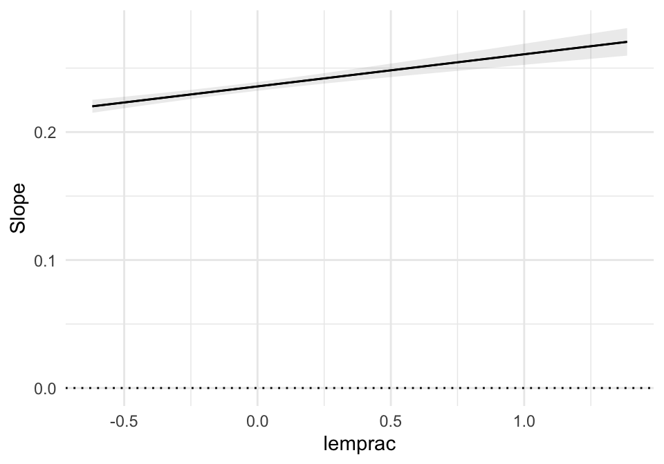

22.4 Lecture Assignment

In the turnout model (A.1), write the fitted line for ss = 0 and ss = 1. Identify the slope in each case.
In the TV16 model (B.1), interpret the interaction sign: does ideology matter more or less among college-educated respondents?
Pick two values of the continuous variable (e.g., ideo=2 and ideo=4). Compute the predicted probability for college vs non-college using the estimated coefficients and compare.